What Electron Affinity Explains Atomic Energy Behavior
Table of Contents
- Electron Affinity: Definition, Quantification, and Comparative Analysis in the Periodic Table
- Definition and Core Concept of Electron Affinity
- Quantitative Trends: Electron Affinity Values for Group 1 and Group 17 Elements
- Distinction Between Electron Affinity and Ionization Energy
- Factors Influencing Electron Affinity Trends in the Periodic Table
- Atomic Radius and Electron-Nucleus Attraction
- Nuclear Charge and Effective Nuclear Charge (Z eff )
- Electron Shielding and Subshell Effects
- Electron-Electron Repulsion in Multi-Electron Atoms
- Flowchart: Electron Affinity Trends Across the Periodic Table
- Experimental Conditions Affecting Measured Electron Affinity
- Electron Affinity and Chemical Reactivity
- Correlation Between Electron Affinity and Nonmetal Reactivity
- Comparative Analysis of Halogen Reactivity Across Periods
- Real-World Applications of High Electron Affinity
- Predicting Reaction Spontaneity Using Electron Affinity Data
- Exceptions and Anomalies in Electron Affinity
- Major Exceptions to Electron Affinity Trends
- Oxygen’s Lower Electron Affinity Than Sulfur: Orbital Repulsion and Atomic Structure
- Comparative Analysis: Nitrogen vs. Phosphorus Electron Affinity
- Predicting Electron Affinity Anomalies Using Molecular Orbital Theory
- Experimental Methods for Measuring Electron Affinity
- Electron Attachment Spectroscopy
- Born-Haber Cycle for Indirect Electron Affinity Calculation
- Comparison of Experimental Techniques for Electron Affinity Measurement
- Franck-Condon Principle in Electron Affinity Spectroscopy
- FAQ
- Why does electron affinity generally decrease as you move down a group in the periodic table?
- What is electron affinity in chemistry?
- What does electron affinity mean?
- What is electron affinity in chemistry for class 11 students?
- What is the difference between electron affinity and electronegativity?
- How does electron affinity compare to electronegativity?
Electron affinity represents a fundamental yet often underappreciated property in chemistry—the energy change accompanying an electron’s addition to a neutral atom. This metric, quantified in kilojoules per mole, governs reactivity, bonding stability, and material design, from ionic compounds to advanced semiconductors. Unlike ionization energy, which measures electron removal, electron affinity reveals how readily atoms accept electrons, shaping periodic trends and industrial applications alike.
The concept bridges theoretical principles—such as atomic radius, nuclear charge, and electron configuration—and practical outcomes, including the efficiency of batteries or the doping of silicon. By examining exceptions like noble gases or the anomalous behavior of oxygen, scientists uncover deeper insights into molecular stability and reaction spontaneity. Experimental techniques, from spectroscopy to Born-Haber cycles, further refine these measurements, ensuring accuracy in both academic research and technological innovation.
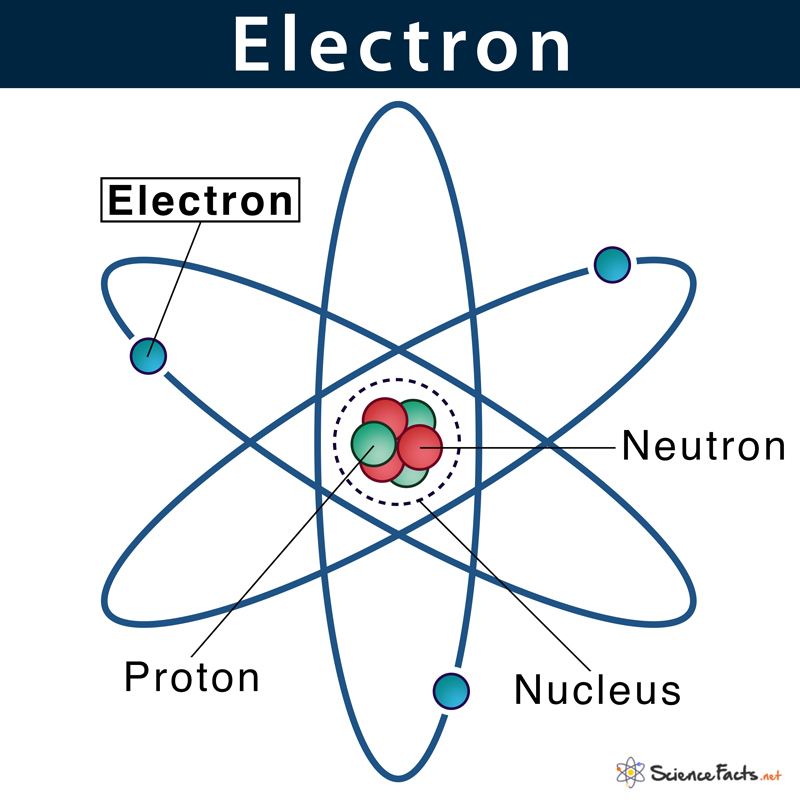
Electron Affinity: Definition, Quantification, and Comparative Analysis in the Periodic Table
Electron affinity (EA) is a fundamental thermodynamic property in chemistry that quantifies the energy change accompanying the addition of an electron to a neutral atom in its gaseous state. Unlike ionization energy, which measures the energy required to remove an electron, electron affinity reflects the atom’s propensity to attract and accommodate an additional electron, influencing chemical reactivity, bonding, and periodic trends. The magnitude and sign of electron affinity provide critical insights into an element’s stability, electronegativity, and tendency to form anions. This discussion elucidates its precise definition, units of measurement, and comparative trends across the periodic table, with a focus on Group 1 and Group 17 elements, while distinguishing it from ionization energy through structured data comparisons.Definition and Core Concept of Electron Affinity
Electron affinity is defined as the energy change (ΔE) when a neutral atom in the gaseous phase gains an electron to form a monatomic anion (X(g) + e⁻ → X⁻(g)). This process can be either exothermic (releasing energy, ΔE < 0) or endothermic (requiring energy input, ΔE > 0), depending on the atom’s electronic configuration and nuclear charge. Exothermic electron affinities indicate a favorable electron gain, typically observed in nonmetals with high effective nuclear charge or stable half-filled or fully filled subshells. Conversely, endothermic values suggest repulsion between the incoming electron and existing electron density, often seen in atoms with filled valence shells (e.g., noble gases) or those where electron pairing disrupts stability.The units of electron affinity are universally expressed in kilojoules per mole (kJ/mol), aligning with standard thermodynamic conventions. A negative EA value (e.g., −328 kJ/mol for chlorine) signifies an exothermic process, while a positive value (e.g., +74 kJ/mol for beryllium) denotes endothermic behavior. The sign convention distinguishes electron affinity from ionization energy, where positive values indicate energy absorption (endothermic) and negative values are not applicable. For example:
Electron Affinity (EA): X(g) + e⁻ → X⁻(g) + EA (kJ/mol)
Ionization Energy (IE): X(g) → X⁺(g) + e⁻ − IE (kJ/mol)
Quantitative Trends: Electron Affinity Values for Group 1 and Group 17 Elements
Electron affinity exhibits periodic trends governed by atomic radius, nuclear charge, and electron shielding. Group 1 (alkali metals) and Group 17 (halogens) display contrasting behaviors due to their electronic configurations. Alkali metals, with a single valence electron in an ns¹ orbital, exhibit positive or slightly negative electron affinities because adding an electron disrupts their stable configuration, requiring energy input. Halogens, with one electron short of a noble gas configuration (ns²np⁵), demonstrate highly exothermic electron affinities due to the strong attraction for an additional electron to achieve stability.The following table compares electron affinity values (in kJ/mol) for select elements in these groups, illustrating the trend toward more negative values as nuclear charge increases within a period:
| Group | Element | Electron Affinity (kJ/mol) | Trend Explanation |
|---|---|---|---|
| Group 1 (Alkali Metals) | Lithium (Li) | −60 | Low nuclear charge; added electron pairs with existing 2s¹, causing repulsion. |
| Sodium (Na) | −53 | Larger atomic radius reduces effective nuclear attraction. | |
| Potassium (K) | −48 | Further reduced attraction due to increased shielding by inner electrons. | |
| Rubidium (Rb) | −47 | Minimal change; electron affinity approaches near-zero for heavier alkali metals. | |
| Group 17 (Halogens) | Fluorine (F) | −328 | Highest EA in the periodic table; small size and strong nuclear attraction. |
| Chlorine (Cl) | −349 | Larger atomic radius than fluorine reduces electron-electron repulsion in the 3p⁵ subshell. | |
| Bromine (Br) | −325 | Slightly less exothermic due to increased atomic size and shielding. | |
| Iodine (I) | −295 | Weaker attraction; larger radius and diffuse electron cloud reduce EA magnitude. |
Distinction Between Electron Affinity and Ionization Energy
While both electron affinity and ionization energy describe energy changes associated with electron transfer, they represent opposite processes and differ in thermodynamic sign conventions, atomic behavior, and periodic trends. The following table highlights their key distinctions:| Property | Electron Affinity (EA) | Ionization Energy (IE) | ||||||||||||||||||||||||||||
|---|---|---|---|---|---|---|---|---|---|---|---|---|---|---|---|---|---|---|---|---|---|---|---|---|---|---|---|---|---|---|
| Process | Addition of an electron to a neutral atom: X(g) + e⁻ → X⁻(g) | Removal of an electron from a neutral atom: X(g) → X⁺(g) + e⁻ | ||||||||||||||||||||||||||||
| Energy Sign Convention | Negative (exothermic) if energy is released; positive (endothermic) if energy is absorbed. | Always positive (endothermic); energy is required to overcome nuclear attraction. | ||||||||||||||||||||||||||||
| Periodic Trends |
|
|
||||||||||||||||||||||||||||
| Chemical Implications |
|
|
||||||||||||||||||||||||||||
| Units and Measurement | kJ/mol; can be positive or negative. | kJFactors Influencing Electron Affinity Trends in the Periodic TableElectron affinity (EA) reflects the energy change when an electron is added to a neutral atom in the gaseous state, forming a negative ion. The trends in EA across the periodic table are governed by electrostatic interactions, quantum mechanical effects, and atomic structure. Key determinants include nuclear charge, atomic radius, electron shielding, and electron configuration stability. These factors collectively dictate whether an atom readily accepts an electron, exhibits exothermic or endothermic EA, or deviates from expected patterns due to electron-electron repulsion or filled subshell effects.The variation in EA across periods and groups is not strictly linear due to competing influences such as electron repulsion in multi-electron systems and the stability of half-filled or fully filled subshells. Below, the interplay of these factors is dissected, followed by a comparative analysis of trends and exceptions, including experimental conditions that modify measured values. Atomic Radius and Electron-Nucleus AttractionThe atomic radius directly influences electron affinity by determining the distance between the incoming electron and the nucleus. A smaller atomic radius increases the effective nuclear charge experienced by the added electron, enhancing attractive forces and typically resulting in higher (more negative) EA values.For example, in Group 17 (halogens), fluorine (F) has the smallest atomic radius among its group, leading to a high EA (−328 kJ/mol). However, chlorine (Cl) exhibits a slightly less negative EA (−349 kJ/mol) due to increased electron-electron repulsion in its smaller 2p subshell compared to the larger 3p subshell of Cl. Conversely, in Group 1 (alkali metals), larger atomic radii (e.g., cesium, Cs) reduce nuclear attraction, yielding low or even positive EA values (e.g., Cs: ~46 kJ/mol), indicating reluctance to gain an electron. Key Relationships: Nuclear Charge and Effective Nuclear Charge (Zeff)The nuclear charge (Z) increases across periods (left to right) due to the addition of protons, while electron shielding by inner-shell electrons remains relatively constant. This results in a higher effective nuclear charge (Zeff) for valence electrons, which strengthens their attraction to the nucleus and generally increases EA.However, Group 2 elements (alkaline earth metals) and noble gases exhibit anomalies: Quantitative Insight: Zeff = Z − Swhere S is the shielding constant. Higher Zeff correlates with more negative EA, except where subshell stability dominates. Electron Shielding and Subshell EffectsElectron shielding by inner-shell electrons reduces the net attraction between the nucleus and the added electron, thereby moderating EA trends. This effect is more pronounced in atoms with larger atomic radii, where valence electrons are farther from the nucleus.Periodic Trends: Example of Shielding Impact: Electron-Electron Repulsion in Multi-Electron AtomsIn atoms with multiple electrons, repulsion between valence electrons can reduce EA by destabilizing the added electron. This effect is particularly significant in small atoms with high electron density, such as Group 16 elements (O, S, Se).Notable Cases: Quantitative Explanation: Erep ∝ 1/ravgwhere ravg is the average distance between electrons. Smaller ravg (e.g., in O) increases Erep, reducing EA. Flowchart: Electron Affinity Trends Across the Periodic TableBelow is a conceptual flowchart illustrating EA variations, with annotations for exceptions. The diagram follows two axes:1. Horizontal (Periods): Left to right (increasing Z). 2. Vertical (Groups): Top to bottom (increasing atomic radius). Key Annotations: - Exceptions: Visual Representation (Descriptive): Periods (Left → Right): Groups (Top → Bottom): Experimental Conditions Affecting Measured Electron AffinityElectron affinity values are derived from experimental measurements, which are sensitive to environmental factors
Electron Affinity and Chemical ReactivityElectron affinity (EA) serves as a quantitative measure of an atom’s propensity to gain an electron, directly influencing its reactivity, particularly in nonmetals where anion formation dominates redox processes. High electron affinity correlates with strong oxidizing power, as seen in halogens and chalcogens, which readily accept electrons to achieve stable electronic configurations. This reactivity underpins critical industrial and technological applications, from battery design to semiconductor doping. Below, the relationship between electron affinity and chemical behavior is examined, including comparative trends across the periodic table and practical implications in redox reactions.Correlation Between Electron Affinity and Nonmetal ReactivityNonmetals with high electron affinities exhibit pronounced reactivity in redox reactions, where they act as oxidizing agents by gaining electrons to form anions. Halogens (Group 17) and chalcogens (Group 16) demonstrate this trend most distinctly due to their proximity to achieving noble gas configurations. For instance, fluorine (EA = −328 kJ/mol) and chlorine (EA = −349 kJ/mol) readily form halide ions (F⁻, Cl⁻) in reactions with metals or other reducing agents, driving processes like the formation of ionic salts (e.g., NaCl) or covalent compounds (e.g., HCl). Similarly, chalcogens such as oxygen (EA = −141 kJ/mol) and sulfur (EA = −200 kJ/mol) participate in redox cycles, forming oxides (O²⁻) or sulfides (S²⁻) in reactions with electropositive elements.The spontaneity of these reactions is governed by the Born-Haber cycle, where electron affinity contributes to the overall lattice energy of the resulting ionic compound. A higher (more negative) electron affinity lowers the activation energy for anion formation, thereby increasing the reaction’s favorability. For example, the reaction of sodium (Na) with chlorine (Cl₂) to form NaCl is highly exothermic (−411 kJ/mol) due to chlorine’s strong electron affinity, which stabilizes the Cl⁻ ion and compensates for sodium’s ionization energy. Comparative Analysis of Halogen Reactivity Across PeriodsElectron affinity trends within groups reveal periodic variations that influence reactivity. Halogens in the same group (e.g., fluorine vs. iodine) exhibit decreasing electron affinities with increasing atomic size, as the added electron experiences greater shielding and weaker nuclear attraction. This trend is reflected in their reactivity:- Fluorine (F₂): Highest electron affinity (−328 kJ/mol) and strongest oxidizing agent among halogens. It displaces other halides from solution (e.g., F₂ + 2NaBr → 2NaF + Br₂) due to its ability to pull electrons aggressively, even from weaker oxidizing agents like bromine. This periodicity explains why fluorine is the most reactive halogen in displacement reactions, while iodine’s weaker electron affinity restricts its role to milder redox processes. The halogen displacement series (F₂ > Cl₂ > Br₂ > I₂) directly mirrors their electron affinities, with higher EA correlating to stronger oxidizing ability. Real-World Applications of High Electron AffinityElements with high electron affinities are pivotal in technologies where electron transfer drives functionality. Key applications include:Battery Cathodes: Lithium-ion batteries rely on cathode materials (e.g., LiCoO₂, LiFePO₄) where transition metals with high electron affinities (e.g., cobalt, manganese) stabilize the oxide lattice during lithium intercalation. The strong EA of oxygen (−141 kJ/mol) ensures robust anion-cation interactions, enhancing ionic conductivity and cycle life. Phosphorus-doped silicon (used in lithium-ion anodes) leverages phosphorus’s EA (−72 kJ/mol) to improve electron mobility, mitigating capacity fade.In both cases, electron affinity dictates the efficiency of charge separation and transport, directly impacting device performance. For example, lithium-ion batteries with cathodes incorporating elements like nickel (EA = −119 kJ/mol) achieve higher energy densities by balancing electron affinity with structural stability. Predicting Reaction Spontaneity Using Electron Affinity DataThe spontaneity of ionic compound formation (e.g., NaCl) can be predicted by integrating electron affinity with lattice energy (U) and ionization energy (IE) via the Born-Haber cycle. Below is a step-by-step procedure:
Exceptions and Anomalies in Electron AffinityElectron affinity trends across the periodic table generally follow predictable patterns, such as increasing values from left to right within a period and decreasing trends down a group. However, deviations from these trends—referred to as exceptions or anomalies—arise due to electronic configurations, orbital stability, and interelectronic repulsion effects. These anomalies provide critical insights into atomic structure and reactivity, particularly in elements where half-filled or fully filled subshells confer unusual stability. Below, the three primary exceptions—noble gases, Group 2 elements, and second-period elements—are analyzed, followed by a mechanistic explanation for oxygen’s lower electron affinity compared to sulfur, supported by orbital diagrams, comparative data, and molecular orbital theory.Major Exceptions to Electron Affinity TrendsThree key exceptions disrupt the expected increase in electron affinity across periods, primarily due to electronic stability and repulsion effects.Noble Gases: Zero or Near-Zero Electron Affinity Group 2 Elements: Low Electron Affinity Due to Filled s-Subshells Second-Period Elements: Nitrogen and Oxygen Anomalies Oxygen’s Lower Electron Affinity Than Sulfur: Orbital Repulsion and Atomic StructureThe electron affinity of oxygen (141 kJ/mol) is lower than that of sulfur (200 kJ/mol), despite oxygen’s higher nuclear charge. This anomaly arises from electron-electron repulsion in the compact 2p subshell of oxygen, which is mitigated in sulfur’s larger 3p subshell.Orbital Diagram Explanation In sulfur, the 3p subshell is larger, reducing electron density and minimizing repulsion when an electron is added: Quantitative Comparison This trend is consistent across the periodic table: second-period elements often exhibit lower electron affinities than their heavier counterparts due to the compactness of their valence orbitals. Comparative Analysis: Nitrogen vs. Phosphorus Electron AffinityNitrogen and phosphorus exhibit contrasting electron affinities due to differences in orbital stability and electron pairing. Nitrogen’s half-filled p subshell (2p³) is particularly stable, while phosphorus’s 3p³ configuration is less so, leading to distinct reactivity patterns.Electron Configurations and Affinities
Predicting Electron Affinity Anomalies Using Molecular Orbital TheoryMolecular orbital (MO) theory provides a framework for predicting electron affinity anomalies in diatomic molecules, particularly for small systems like O₂ and S₂. The presence of antibonding orbitals and their occupancy influence electron addition trends.Role of Antibonding Orbitals in O₂ vs. S₂ Quantitative Impact on Electron Affinity General Prediction Rule
Experimental Methods for Measuring Electron AffinityElectron affinity (EA) quantifies the energy change when a neutral atom or molecule in the gaseous state gains an electron to form a negative ion. Experimental determination of EA requires precise techniques capable of resolving minute energy variations, often below 1 eV. Methods range from direct spectroscopic observations of electron attachment to indirect thermodynamic cycles, each offering distinct advantages and limitations. This section examines three primary experimental approaches—electron attachment spectroscopy, thermal measurements via the Born-Haber cycle, and photoelectron spectroscopy—highlighting their underlying principles, instrumentation, and applications in periodic trend analysis.Electron Attachment SpectroscopyElectron attachment spectroscopy directly measures the energy released or absorbed when low-energy electrons interact with gaseous atoms or molecules, producing negative ions. The method relies on mass spectrometers to detect the resulting ions while tuning electron beam energies to identify resonance conditions corresponding to electron affinity.Equipment and Principles The detection of negative ions occurs when the electron beam energy matches the EA value, producing a sharp increase in ion signal. For example, in chlorine (EA = 3.61 eV), a peak in the ion yield at 3.61 eV confirms the electron attachment energy. The Franck-Condon principle governs the transition: vertical excitation (no nuclear rearrangement) dominates, as electronic transitions occur faster than atomic vibrations, leading to discrete spectral features. Key Considerations Born-Haber Cycle for Indirect Electron Affinity CalculationThe Born-Haber cycle provides an indirect route to determine EA by linking thermodynamic data of ionic solid formation to lattice energy, sublimation enthalpy, and ionization energy. For instance, the formation of sodium fluoride (NaF) illustrates this approach:Steps and Thermodynamic Relationships 2. Solving for EA(F): Advantages and Constraints Comparison of Experimental Techniques for Electron Affinity MeasurementThe following table contrasts three primary methods—electron attachment spectroscopy, thermal measurements via Born-Haber cycles, and photoelectron spectroscopy—across key dimensions:
Franck-Condon Principle in Electron Affinity SpectroscopyThe FranckElectron affinity is more than a numerical value; it is a lens through which chemists decode atomic behavior, predict reactivity, and engineer materials with precision. From the high electron affinity of halogens driving anion formation to the anomalies in second-period elements exposing orbital complexities, this property underpins both foundational chemistry and cutting-edge applications. Mastering electron affinity trends not only clarifies periodic table patterns but also equips researchers to optimize processes—whether in energy storage, catalysis, or semiconductor fabrication—where electron transfer dictates performance. Understanding its nuances transforms theoretical knowledge into actionable insights for science and industry. FAQWhy does electron affinity generally decrease as you move down a group in the periodic table?Electron affinity decreases down a group because the outermost electrons are farther from the nucleus, experiencing weaker attraction and less energy gain when added. Additionally, the increased atomic size and shielding by inner electrons reduce the effective nuclear charge, making it less favorable to attract an extra electron. What is electron affinity in chemistry?Electron affinity is the energy change that occurs when an isolated gaseous atom gains an electron to form a negative ion. It is typically measured in kJ/mol and can be either exothermic (releasing energy, negative value) or endothermic (absorbing energy, positive value), depending on the atom’s tendency to accept an electron. What does electron affinity mean?Electron affinity refers to how readily an atom accepts an additional electron. A high (more negative) electron affinity indicates a strong attraction for the extra electron, while a low or positive value suggests the atom resists gaining an electron, often due to electron-electron repulsion or a stable electron configuration. What is electron affinity in chemistry for class 11 students?Electron affinity is the energy released or absorbed when a neutral atom in the gaseous state gains an electron to become a negatively charged ion. For class 11, it’s important to note that most nonmetals (like halogens) have high electron affinities, while noble gases and some metals have low or positive values due to stable or unfavorable electron configurations. What is the difference between electron affinity and electronegativity?Electron affinity is the energy change when an atom gains an electron (a quantitative measure of attraction for an extra electron), while electronegativity is a qualitative measure of an atom’s ability to attract shared electrons in a bond. Both relate to atomic pull on electrons, but electron affinity focuses on isolated atoms, while electronegativity applies to bonded atoms (e.g., in covalent bonds). How does electron affinity compare to electronegativity?Electron affinity measures the energy released when an atom gains an electron in isolation, while electronegativity ranks an atom’s ability to pull shared electrons toward itself in a chemical bond. Trends differ slightly: electron affinity often peaks at halogens, while electronegativity follows a smoother trend (e.g., fluorine is most electronegative but has a lower electron affinity than chlorine due to electron repulsion in its small size). |
Leave a Comment
Comments are moderated before appearing. The data you submit is processed according to the Privacy Policy of Voltefac.