What Is The Determinant Of A Matrix And Its Fundamental Role
Table of Contents
- Definition and Core Concept of Determinants
- Mathematical Definition and Role in Square Matrices
- Calculation of the Determinant for a 2×2 Matrix
- Comparison of Determinant with Other Matrix Properties
- Derivation of the Determinant for a 3×3 Matrix
- Computational Methods and Algorithms for Determinant Calculation
- Laplace Expansion and Recursive Computation
- Computational Methods Comparison
- Determinant Calculation via Row Reduction (Gauss Elimination)
- Geometric and Physical Interpretations of Determinants
- Determinant as a Scaling Factor in Linear Transformations
- Effect of Matrix Operations on Determinants
- Determinant and the Cross Product in 3D
- Computing Area and Volume via Determinants
- Comparative Table: Determinant in 2D and 3D Transformations
- Applications in Linear Algebra and Beyond
- Solving Systems of Linear Equations via Cramer’s Rule
- Eigenvalue Problems and the Characteristic Polynomial
- Applications in Computer Graphics and Physics
- Probability Theory and Multivariate Distributions
- Optimization: Quadratic Forms and Constrained Systems
- Advanced Topics and Special Cases in Determinant Theory
- Blockwise Determinant Formula and Applicability Conditions
- Determinants of Symmetric, Skew-Symmetric, and Orthogonal Matrices
- Permanents and Their Contrast with Determinants
- Determinants in Lie Algebras and Differential Geometry
- FAQ
- What is the determinant of a matrix used for?
- What is the determinant of a matrix in simple terms?
- What does the determinant of a matrix mean?
- How do you calculate the determinant of a 3x3 matrix?
- What is the determinant of a matrix and why is it important?
- How is the determinant of a matrix used in linear algebra?
The determinant of a matrix is a scalar value that encapsulates critical properties of square matrices, serving as a cornerstone in linear algebra with applications spanning geometry, physics, and computational science. Beyond its role in assessing matrix invertibility, it quantifies the scaling factor of linear transformations—whether expanding areas in two dimensions or volumes in three-dimensional space. This foundational concept not only underpins solutions to linear systems via Cramer’s Rule but also bridges abstract theory with tangible geometric interpretations, such as the orientation and magnitude of vector transformations.
From the straightforward calculation of 2×2 determinants to the recursive methods for n×n matrices, the determinant’s computation evolves alongside its theoretical depth. Its interplay with eigenvalues, cross products, and even advanced topics like Lie algebras demonstrates its versatility, while numerical challenges in large-scale computations highlight the need for optimized algorithms. By exploring its definitions, geometric significance, and real-world applications—ranging from computer graphics to probability—the determinant emerges as a unifying tool in mathematical analysis, bridging pure theory with practical problem-solving.

Definition and Core Concept of Determinants
The determinant is a scalar value uniquely associated with a square matrix, serving as a fundamental invariant in linear algebra with applications in solving systems of linear equations, evaluating matrix invertibility, and computing eigenvalues. Unlike other matrix properties such as the trace or eigenvalues, the determinant provides a concise measure of the matrix’s geometric transformation effects, including area/volume scaling and orientation preservation. Its calculation varies in complexity depending on matrix size, with distinct methods for 2×2, 3×3, and larger matrices.The determinant’s geometric interpretation extends beyond algebra, offering insights into linear transformations. For instance, a determinant of zero indicates a collapsed transformation (singular matrix), while a positive or negative value reflects volume preservation or reversal, respectively. This dual role—algebraic and geometric—makes the determinant indispensable in fields ranging from physics to computer graphics.
Mathematical Definition and Role in Square Matrices
A determinant is defined for any n×n square matrix A = [aᵢⱼ] as a scalar computed via a sum of products of matrix elements, incorporating permutations of column indices. For a matrix to possess a determinant, it must be square, as non-square matrices lack a unique scaling factor for their transformations. The determinant’s primary roles include:The determinant’s algebraic definition for an n×n matrix A is:
det(A) = Σ (–1)^σ · a₁,σ(1) · a₂,σ(2) · ... · aₙ,σ(n)This formula generalizes to higher dimensions but becomes computationally intensive for large n, necessitating recursive methods like Laplace expansion.
where the sum is over all permutations σ of {1, 2, ..., n}, and (–1)^σ denotes the sign of the permutation (even or odd).
Calculation of the Determinant for a 2×2 Matrix
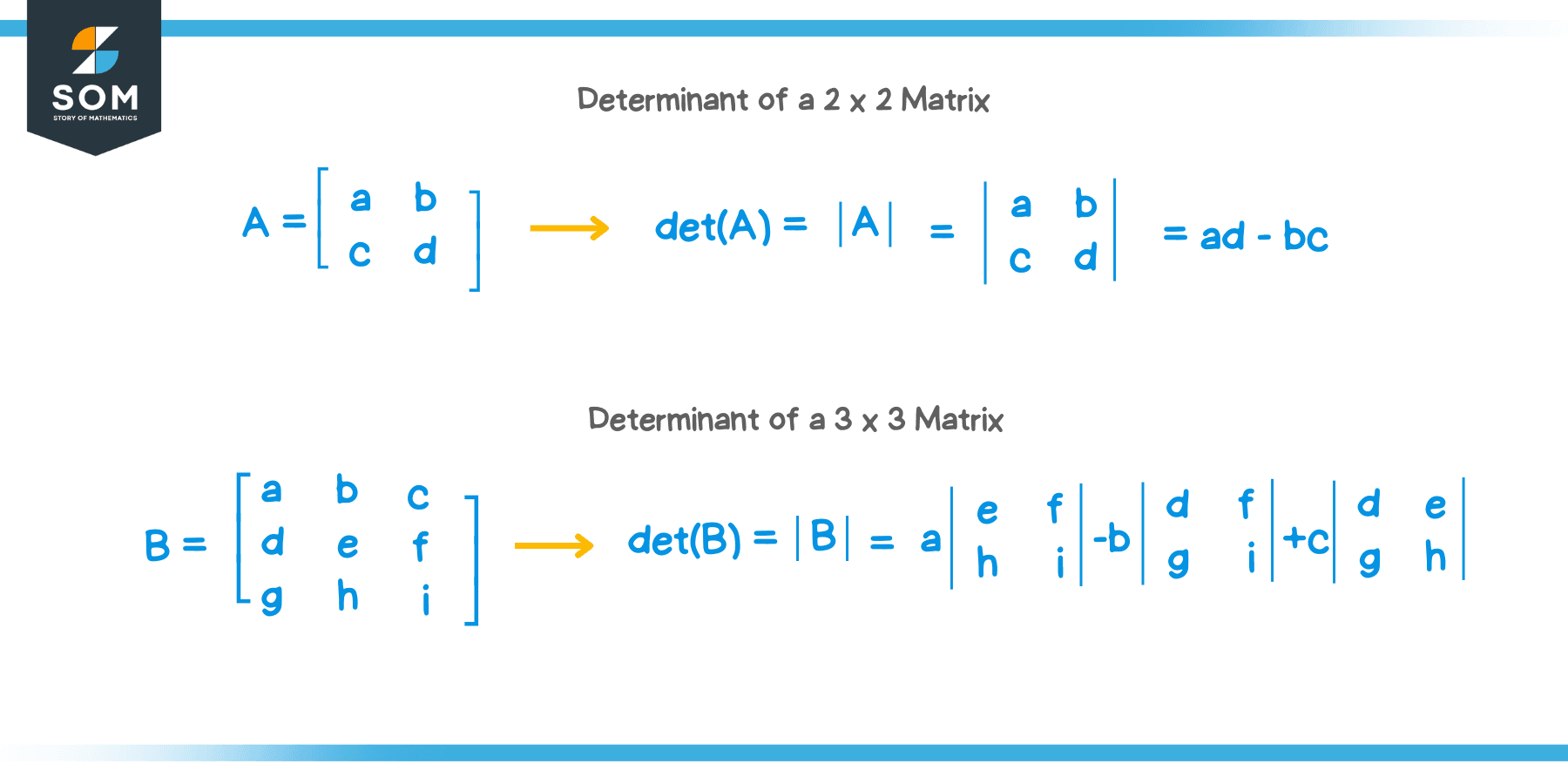
The determinant of a 2×2 matrix A = [a b; c d] is computed using the formula:det(A) = ad – bcThis expression arises from the general definition by considering the two permutations of column indices (identity and swap), where:
Geometric Interpretation:
For a linear transformation represented by A, the determinant ad – bc scales the area of the unit square in ℝ². If det(A) = 0, the transformation collapses the plane into a line or point (e.g., A = [1 2; 2 4] maps all vectors to the line y = 2x). If det(A) = 1, the transformation preserves area (e.g., rotation matrices).
Example:
For A = [3 1; 2 4], det(A) = (3)(4) – (1)(2) = 12 – 2 = 10. The unit square’s area is scaled by 10 under this transformation.
Comparison of Determinant with Other Matrix Properties
The determinant, trace, and eigenvalues are distinct yet interrelated properties of square matrices. Below is a comparative analysis highlighting their roles and differences:| Property | Definition | Key Role | Computational Complexity | Geometric Interpretation | Invertibility Condition |
|---|---|---|---|---|---|
| Determinant | Scalar sum of signed products of matrix elements (permutations). | Tests invertibility; measures volume scaling. | O(n!) for general case; O(n³) via LU decomposition. | Absolute value = scaling factor; sign = orientation. | det(A) ≠ 0. |
| Trace | Sum of diagonal elements: tr(A) = Σ aᵢᵢ. | Sum of eigenvalues; invariant under similarity transformations. | O(n). | No direct geometric interpretation. | No direct invertibility test. |
| Eigenvalues | Scalars λ satisfying det(A – λI) = 0. | Characterize linear transformations; diagonalization. | O(n³) for computation (e.g., QR algorithm). | Magnitude = scaling factor; angle = rotation. | No zero eigenvalue ⇒ invertible. |
Derivation of the Determinant for a 3×3 Matrix
The determinant of a 3×3 matrix A = [a b c; d e f; g h i] can be computed using the Rule of Sarrus (for small matrices) or Laplace expansion (general method). Both methods rely on sign alternation based on permutation parity.Rule of Sarrus (Visual Method):
Extend the matrix by repeating the first two columns, then sum the products of diagonals with alternating signs:
det(A) = (a·e·i + b·f·g + c·d·h) – (c·e·g + a·f·h + b·d·i)Steps:
1. Multiply the three main diagonals (left to right): a·e·i, b·f·g, c·d·h.
2. Multiply the three anti-diagonals (right to left): c·e·g, a·f·h, b·d·i.
3. Subtract the sum of anti-diagonals from the sum of main diagonals.
Example:
For A = [1 2 3; 4 5 6; 7 8 9]:
det(A) = (1·5·9 + 2·6·7 + 3·4·8) – (3·5·7 + 1·6·8 + 2·4·9)
= (45 + 84 + 96) – (105 + 48 + 72)
= 225 – 225 = 0.
This matrix is singular (non-invertible), as expected for a matrix with linearly dependent rows/columns.
Laplace Expansion (Cofactor Expansion):
For larger matrices, Laplace expansion reduces the problem to smaller determinants. Expanding along the first row:
det(A) = a·det([e f; h i]) – b·det([d f; g i]) + c·det([d e; g h])Sign Alternation Pattern:
The signs alternate starting with + for the first element (a₁₁), then – for a₁₂, + for a₁₃, etc. This pattern corresponds to the parity of permutations:
Example:
For A = [1 0 2; 3 4 5; 0 1 6], expanding along the first row:
det(A) = 1·det([4 5; 1 6]) – 0·det([3 5; 0 6]) + 2·det([3 4; 0 1])
= 1·(24 –
Computational Methods and Algorithms for Determinant Calculation
The determinant of a matrix is a scalar value that encapsulates critical properties of linear transformations, including invertibility and volume scaling. While its definition provides theoretical insight, practical computation requires efficient algorithms tailored to matrix structure and size. Recursive methods like Laplace expansion offer a foundational approach, but their scalability diminishes for large matrices. Alternative techniques, such as row reduction and decomposition-based methods, leverage numerical stability and computational efficiency. This section examines these methods, their mathematical underpinnings, and their application in real-world scenarios, including challenges posed by floating-point arithmetic and matrix sparsity.
Laplace Expansion and Recursive Computation
The Laplace expansion (or cofactor expansion) computes the determinant of an n×n matrix by recursively decomposing it into smaller submatrices. For a matrix A, the determinant is expressed as:
\[
Key Observations:
\det(A) = \sum_{j=1}^{n} (-1)^{1+j} a_{1j} \det(M_{1j})
\]
where \(a_{1j}\) is the element in the first row and j-th column, and \(M_{1j}\) is the corresponding minor (submatrix obtained by removing the first row and j-th column).
Computational Complexity:
The naive recursive implementation has a time complexity of \(O(n!)\), as it evaluates \(n\) subdeterminants of size \(n-1\), each requiring \(n-1\) evaluations, and so on. This makes it impractical for matrices larger than \(4 \times 4\) without optimizations.
Optimization Strategies:
Computational Methods Comparison
The choice of method depends on matrix properties (size, sparsity, symmetry) and computational constraints. Below is a comparative table of common approaches:| Method | Description | Time Complexity | Space Complexity | Use Cases | Numerical Stability |
|---|---|---|---|---|---|
| Laplace Expansion | Recursive cofactor expansion along a row/column. | \(O(n!)\) | \(O(n^2)\) (recursion stack) | Small matrices (\(n \leq 4\)), theoretical analysis. | Low (error propagation in recursion). |
| Gauss-Jordan Elimination | Row operations to transform the matrix into upper triangular form, then multiply diagonal elements. | \(O(n^3)\) | \(O(n^2)\) | General dense matrices, symbolic computation. | Moderate (pivoting mitigates instability). |
| LU Decomposition | Factorizes the matrix into lower (\(L\)) and upper (\(U\)) triangular matrices; \(\det(A) = \prod_{i=1}^{n} u_{ii}\). | \(O(n^3)\) | \(O(n^2)\) | Dense matrices, repeated computations (e.g., solving linear systems). | High (partial pivoting ensures stability). |
| Leibniz Formula | Sum of \(n!\) products of matrix elements, one from each row/column. | \(O(n \cdot n!)\) | \(O(1)\) | Theoretical proofs, small matrices (\(n \leq 3\)). | Low (exponential terms dominate errors). |
| Barrett Reduction | Iterative method for tridiagonal matrices, leveraging recurrence relations. | \(O(n)\) | \(O(1)\) | Tridiagonal or banded matrices. | High (numerically stable for well-conditioned matrices). |
Determinant Calculation via Row Reduction (Gauss Elimination)
Gauss elimination transforms a matrix into row-echelon form (upper triangular) through elementary row operations, after which the determinant is the product of diagonal elements. The process involves:1. Partial Pivoting: Swap rows to place the largest absolute value in the current column’s pivot position, minimizing rounding errors.
2. Row Operations:
Example: 4×4 Matrix Determinant
Consider the matrix:
\[
A = \begin{bmatrix}
2 & 1 & 0 & 1 \\
4 & 3 & 1 & 2 \\
-1 & 0 & 2 & 1 \\
1 & 2 & 1 & 4
\end{bmatrix}
\]
Steps:
1. Pivot Row 1, Column 1:
\text{Row 2} \leftarrow \text{Row 2} - 2 \times \text{Row 1} = [0, 1, 1, 0]
\]
\text{Row 3} \leftarrow \text{Row 3} + 0.5 \times \text{Row 1} = [0, 0.5, 2, 1.5]
\]
\text{Row 4} \leftarrow \text{Row 4} - 0.5 \times \text{Row 1} = [0, 1.5, 1, 3.5]
\]
\begin{bmatrix}
2 & 1 & 0 & 1 \\
0 & 1 & 1 & 0 \\
0 & 0.5 & 2 & 1.5 \\
0 & 1.5 & 1 & 3.5
\end{bmatrix}
\]
2. Pivot Row 2, Column 2:
\text{Row 3} \leftarrow \text{Row 3} - 0.5 \times \text{Row 2} = [0, 0, 1.5, 0.75]
\]
\text{Row 4} \leftarrow \text{Row 4} - 1.5 \times \text{Row 2} = [0, 0, -0.5, 3.5]
\]
\begin{bmatrix}
2 & 1 & 0 & 1 \\
0 & 1 & 1 & 0 \\
0 & 0 &
Geometric and Physical Interpretations of Determinants
The determinant of a matrix transcends its algebraic definition, offering profound geometric and physical insights into linear transformations. It quantifies how a matrix scales, shears, or rotates space, revealing intrinsic properties such as orientation preservation, singularity, and volume/area distortion. This section explores these interpretations through dimensional analysis, operational effects on determinants, and their connections to fundamental geometric constructs like the cross product and parallelepiped volumes.Determinant as a Scaling Factor in Linear Transformations
The determinant measures the factor by which a linear transformation expands or contracts volumes (in 3D) or areas (in 2D) under the action of the matrix. For a matrix A, the absolute value of its determinant, |det(A)|, represents the scaling factor applied to the unit hypercube (or standard basis vectors) after transformation.In 2D:
Consider a matrix A = [a b; c d] acting on the unit square formed by vectors e₁ = (1, 0) and e₂ = (0, 1). The transformed vectors are:
Ae₁ = (a, c) and Ae₂ = (b, d).
The area of the parallelogram formed by these vectors is:
Area = |det(A)| = |ad − bc|.This area is the determinant’s geometric interpretation: the unit square’s area (1) is scaled by |det(A)|.
In 3D:
For a matrix A = [a b c; d e f; g h i], the determinant scales the volume of the unit cube (formed by e₁, e₂, e₃) by |det(A)|. The transformed vectors Ae₁, Ae₂, Ae₃ form a parallelepiped with volume:
Volume = |det(A)|.If det(A) = 0, the transformation collapses the space into a lower dimension (e.g., a plane in 3D), resulting in zero volume.
Effect of Matrix Operations on Determinants
The determinant’s behavior under elementary row/column operations and matrix decompositions provides insight into how transformations alter space. The following properties illustrate these effects:-
The determinant remains unchanged under transposition, i.e., det(A) = det(Aᵀ). This reflects the symmetry between row and column operations in linear algebra.
det(A) = det(Aᵀ).Row swaps multiply the determinant by −1, indicating a reversal of orientation (e.g., a reflection). For example:
det([a b; c d]) = ad − bc,Scaling a row by λ multiplies the determinant by λ. If a row is scaled by zero, the determinant becomes zero, signifying a singular transformation (e.g., projection onto a plane in 3D).
det([c d; a b]) = −(ad − bc).
Adding a multiple of one row to another leaves the determinant unchanged, as this operation preserves the volume/area of the parallelepiped formed by the transformed basis vectors.
Matrix multiplication satisfies det(AB) = det(A)·det(B), meaning the combined transformation’s scaling factor is the product of individual scaling factors. For instance, a rotation followed by a scaling matrix yields a determinant equal to the product of their determinants.
Determinant and the Cross Product in 3D
In three-dimensional space, the determinant of a matrix formed by three vectors u, v, and w as columns is equal to the scalar triple product u · (v × w), which represents the signed volume of the parallelepiped spanned by the vectors. This relationship is expressed as:det([u v w]) = u · (v × w) = |u||v||w| √(1 − cos²θ₁ − cos²θ₂ − cos²θ₃ + 2cosθ₁cosθ₂cosθ₃),where θ₁, θ₂, and θ₃ are the angles between the vectors. The absolute value yields the volume, while the sign indicates orientation (right-handed or left-handed system).
Example:
For vectors u = (1, 0, 0), v = (0, 1, 0), and w = (0, 0, 1), the determinant is:
det([1 0 0; 0 1 0; 0 0 1]) = 1,which matches the volume of the unit cube and the scalar triple product u · (v × w) = 1.
Computing Area and Volume via Determinants
The determinant provides a direct method to compute the area of a parallelogram or the volume of a parallelepiped formed by column vectors of a matrix. The process involves constructing a matrix with the vectors as columns and evaluating its determinant.Step-by-Step for a Parallelogram (2D):
Given vectors a = (a₁, a₂) and b = (b₁, b₂), the area of the parallelogram they span is:
1. Form the matrix A = [a₁ a₂; b₁ b₂].
2. Compute det(A) = a₁b₂ − a₂b₁.
3. The area is |det(A)|.
Example:
For a = (2, 1) and b = (−1, 3), the area is:
|det([2 1; −1 3])| = |(2)(3) − (1)(−1)| = |6 + 1| = 7.Step-by-Step for a Parallelepiped (3D):
Given vectors a = (a₁, a₂, a₃), b = (b₁, b₂, b₃), and c = (c₁, c₂, c₃), the volume is:
1. Form the matrix A = [a₁ a₂ a₃; b₁ b₂ b₃; c₁ c₂ c₃].
2. Compute det(A).
3. The volume is |det(A)|.
Example:
For a = (1, 0, 0), b = (0, 2, 0), and c = (0, 0, 3), the volume is:
|det([1 0 0; 0 2 0; 0 0 3])| = |1·(2·3 − 0·0) − 0 + 0| = 6.
Comparative Table: Determinant in 2D and 3D Transformations
The following table summarizes the geometric role of the determinant in two and three dimensions, highlighting key distinctions and shared properties.| Property | 2D (Area) | 3D (Volume) | ||||||||||||||||||||||||||||||||||||||
|---|---|---|---|---|---|---|---|---|---|---|---|---|---|---|---|---|---|---|---|---|---|---|---|---|---|---|---|---|---|---|---|---|---|---|---|---|---|---|---|---|
| Geometric Interpretation | Scaling factor for area of the unit square under transformation. | Scaling factor for volume of the unit cube under transformation. | ||||||||||||||||||||||||||||||||||||||
| Zero Determinant | Transformation collapses space into a line (area = 0). | Transformation collapses space into a plane or line (volume = 0). | ||||||||||||||||||||||||||||||||||||||
| Sign of Determinant | Indicates orientation preservation (+) or reversal (−). | Indicates right-handed (+) or left-handed (−) coordinate system. | ||||||||||||||||||||||||||||||||||||||
| Relation to Cross Product | Magnitude of the 2D "cross product" (a₁b₂ − a₂b₁) equals |det(A)|. | Scalar triple product u · (v × w) equals det([u v w]). | ||||||||||||||||||||||||||||||||||||||
| Effect of Scaling | Scaling a row/column by λ scales the area by |λ|. | Scaling a row/column by λ scales the volume by |λ|. | ||||||||||||||||||||||||||||||||||||||
ApplicationsApplications in Linear Algebra and BeyondThe determinant is a fundamental mathematical construct with broad applicability across linear algebra, numerical analysis, physics, and optimization. Beyond its role in characterizing invertibility and volume scaling, determinants provide solutions to linear systems, enable geometric transformations, and underpin advanced computational techniques. Their utility extends to eigenvalue analysis, coordinate transformations, and probabilistic models, making them indispensable in both theoretical and applied mathematics.Determinants serve as a bridge between abstract algebra and practical problem-solving, offering computational efficiency in specific scenarios while revealing deeper structural properties of matrices. Their limitations—such as scalability in large systems—highlight the need for complementary methods, yet their geometric and algebraic interpretations remain foundational in interdisciplinary research. Solving Systems of Linear Equations via Cramer’s RuleCramer’s Rule provides an explicit solution to a system of n linear equations with n variables using determinants. For a system Ax = b, where A is an invertible n × n matrix, the solution for each variable xi is given by:xi = det(Ai) / det(A)Here, Ai is the matrix formed by replacing the i-th column of A with the column vector b. While elegant and computationally straightforward for small systems (n ≤ 3), Cramer’s Rule becomes impractical for large n due to its O(n!) complexity from determinant calculations. For systems exceeding n = 5, iterative methods (e.g., Gaussian elimination) or matrix decomposition techniques (LU, QR) are preferred for efficiency and numerical stability. Limitations in Large Systems: Eigenvalue Problems and the Characteristic PolynomialThe determinant is central to eigenvalue analysis, where it defines the characteristic polynomial of a matrix A:det(A − λI) = 0This polynomial’s roots are the eigenvalues λ1, ..., λn, and their multiplicities determine the matrix’s spectral properties. Determinants also appear in the trace-determinant relationship for the sum and product of eigenvalues: tr(A) = λ1 + ... + λn det(A) = λ1 · ... · λnRole in Diagonalizability: A matrix A is diagonalizable if and only if it has a full set of linearly independent eigenvectors. The determinant ensures non-zero eigenvalues (for invertibility) and influences the algebraic multiplicity of eigenvalues, which must equal their geometric multiplicity for diagonalizability. For defective matrices (where geometric multiplicity < algebraic multiplicity), the Jordan normal form is required, and determinants aid in analyzing such cases via the minimal polynomial. Applications in Computer Graphics and PhysicsDeterminants are pivotal in transformations and coordinate systems, where they quantify scaling factors, orientation preservation, and volume changes. Below is a summary of key applications:
In homogeneous coordinates, a 4×4 transformation matrix M combines translation, rotation, and scaling. The determinant of its linear part (3×3 submatrix) determines whether the transformation preserves, scales, or inverts volume. For instance, a determinant of 0.5 in a scaling matrix compresses space along an axis by half, directly observable in rendered objects. Probability Theory and Multivariate DistributionsDeterminants appear in probability through the density functions of multivariate distributions and volume calculations in high-dimensional spaces. For a multivariate normal distribution with covariance matrix Σ, the probability density function (PDF) includes the determinant of Σ in its normalization:fX(x) = (2π)−n/2 |Σ|−1/2 exp(−½ (x − μ)T Σ−1 (x − μ))Here, |Σ|−1/2 ensures the PDF integrates to 1 over ℝn, with |Σ| representing the generalized variance of the distribution. Volume of the Unit Ball in High Dimensions: Vn = (πn/2 / Γ(n/2 + 1))For n ≥ 5, Vn decreases rapidly due to the determinant-like scaling in spherical coordinates, illustrating how high-dimensional geometry diverges from intuition. This property is critical in stochastic processes (e.g., Monte Carlo integration) and machine learning (e.g., kernel methods). Optimization: Quadratic Forms and Constrained SystemsDeterminants play a role in optimization by characterizing the definiteness of quadratic forms and the feasibility of constrained linear systems. Consider a quadratic form xTAx, where A is symmetric. The sign of the determinant of A (or its principal minors) determines whether the form is positive-definite, negative-definite, or indefinite:- Positive-definite (det(A) > 0): All eigenvalues are positive; the quadratic form is convex. Case Study: Least Squares Optimization with Constraints det([AT A CT; C 0]) ≠ 0Example: Portfolio Optimization In financial mathematics, the Markowitz mean-variance optimization problem minimizes risk (covariance matrix Σ) subject to return constraints. The determinant of Σ appears in the efficient frontier
Advanced Topics and Special Cases in Determinant TheoryThe study of determinants extends beyond fundamental computational methods to encompass specialized matrix structures and theoretical applications in abstract algebra and geometry. Advanced topics reveal deeper connections between linear algebra, combinatorics, and differential geometry, while special cases—such as block matrices, symmetric matrices, and Lie algebraic structures—demonstrate the determinant’s versatility. This section explores these nuanced areas, including blockwise determinant formulas, combinatorial contrasts with permanents, and the role of determinants in Lie derivatives and exterior calculus.Blockwise Determinant Formula and Applicability ConditionsBlock matrices arise naturally in partitioned systems, where a matrix is divided into submatrices (blocks) to simplify analysis. The blockwise determinant formula generalizes the Laplace expansion for square block matrices of the form:\[ where \( A, B, C, D \) are submatrices of compatible dimensions. Under the condition that either \( A \) or \( C \) is invertible, the determinant satisfies: \[ Key conditions for applicability: Example: In control theory, blockwise determinants appear in state-space representations of dynamical systems, where stability analysis relies on the invertibility of \( A \) or \( D \). Determinants of Symmetric, Skew-Symmetric, and Orthogonal MatricesThe determinant exhibits distinct properties for matrices with structural symmetries, reflecting their algebraic and geometric constraints. Below is a comparative table summarizing key patterns:
Permanents and Their Contrast with DeterminantsThe permanent of a matrix \( A \), denoted \( \text{perm}(A) \), is defined as:\[ where \( S_n \) is the symmetric group on \( n \) elements. This resembles the determinant’s Leibniz formula but lacks the sign factor \( (-1)^{\text{sgn}(\sigma)} \). Key Differences: Example: For \( A = \begin{pmatrix} 1 & 1 \\ 1 & 1 \end{pmatrix} \), Determinants in Lie Algebras and Differential GeometryDeterminants play a foundational role in Lie theory and differential geometry, where they quantify infinitesimal transformations and volume preservation.Lie Algebras and Exponential Maps: Exterior Calculus and Lie Derivatives: The determinant of a matrix transcends its role as a mere computational tool, embodying the interplay between algebra and geometry in ways that define the behavior of linear systems. Whether determining the feasibility of solutions, quantifying transformations in multidimensional spaces, or enabling advanced techniques in optimization and physics, its influence is pervasive. As we navigate from basic 2×2 calculations to the intricacies of block matrices and differential geometry, the determinant reveals itself as a fundamental invariant—one that not only resolves theoretical questions but also empowers innovations across disciplines. Its mastery thus remains indispensable for mathematicians, engineers, and scientists seeking to harness the full potential of linear algebra in both abstract and applied contexts. FAQWhat is the determinant of a matrix used for?The determinant measures whether a matrix is invertible (non-zero determinant means invertible) and quantifies scaling factors, orientation, and volume changes under linear transformations. It’s also used in solving systems of linear equations (Cramer’s Rule), computing eigenvalues, and analyzing matrix properties like rank. What is the determinant of a matrix in simple terms?The determinant is a single number calculated from a square matrix that tells you two key things: whether the matrix can be inverted (if it’s zero, it can’t), and how the matrix scales or flips space when applied as a transformation. Think of it as a "health check" for the matrix’s geometric behavior. What does the determinant of a matrix mean?The determinant indicates whether a matrix represents a reversible transformation (non-zero = reversible) and encodes how much area/volume in n-dimensional space is stretched or compressed by the transformation. A zero determinant means the matrix collapses space (e.g., lines or planes map to a single point). How do you calculate the determinant of a 3x3 matrix?For a 3x3 matrix, use the rule of Sarrus or Laplace expansion: subtract the product of diagonals (top-left to bottom-right) from the product of the other diagonal (top-right to bottom-left) for each 2x2 submatrix, then sum the weighted minors. The formula is: What is the determinant of a matrix and why is it important?The determinant is a scalar value derived from a square matrix that reveals its invertibility, geometric effects (scaling/rotation), and stability in systems. It’s crucial for solving linear systems, computing cross products, analyzing eigenvalues, and determining if a matrix preserves or reverses orientation in space. How is the determinant of a matrix used in linear algebra?In linear algebra, the determinant is used to test matrix invertibility, compute eigenvalues (via characteristic polynomials), solve linear systems via Cramer’s Rule, and analyze transformations (e.g., rotations, reflections). It also appears in formulas for matrix adjugates, volumes of parallelepipeds, and the change-of-basis determinant in multilinear algebra. |

Leave a Comment
Comments are moderated before appearing. The data you submit is processed according to the Privacy Policy of Voltefac.