What Is A Polynomial Function Explained Comprehensively
Table of Contents
- Definition and Core Characteristics of Polynomial Functions
- Formal Definition and Algebraic Notation
- Structural Components of Polynomial Functions
- Determining the Degree of a Polynomial
- Comparison with Other Function Types
- Graphical Representation and Behavior of Polynomial Functions
- Step-by-Step Guide to Sketching Polynomial Graphs
- Summary of Graphical Features for Polynomials of Degrees 1–4
- Influence of Coefficients on Graph Shape
- Operations and Manipulations of Polynomial Functions
- Addition, Subtraction, and Multiplication of Polynomials
- Polynomial Division: Long Division and Synthetic Division
- Factoring Polynomials Applications of Polynomial Functions in Real-World Scenarios Polynomial functions serve as fundamental mathematical tools across disciplines, bridging abstract theory with practical problem-solving. Their versatility arises from their ability to model nonlinear relationships, approximate complex behaviors, and optimize systems where linear models fall short. From predicting trajectories in physics to forecasting economic trends, polynomials provide structured frameworks for analyzing dynamic phenomena. This section explores their applications in projectile motion, data trend approximation, economics, and physics, alongside a structured template for solving optimization problems. Modeling Projectile Motion with Polynomial Functions
- Polynomial Approximation of Data Trends: Interpolation vs. Extrapolation
- Economic and Physical Applications of Polynomial Functions
- Template for Solving Real-World Optimization Problems
- Advanced Concepts and Extensions in Polynomial Functions
- The Fundamental Theorem of Algebra and Polynomial Roots
- Polynomial Approximations for Transcendental Functions
- Polynomial Interpolation Methods
- Differentiation and Integration of Polynomial Functions
- Common Mistakes and Troubleshooting in Polynomial Functions
- Frequent Errors in Polynomial Operations
- Troubleshooting Guide for Graphing Polynomial Functions
- Checklist for Verifying Polynomial Solutions
- FAQ-Style Clarifications of Common Misconceptions
- FAQ
- What is a polynomial function in the simplest possible terms?
- How does the graph of a polynomial function look?
- What exactly is a polynomial function in mathematics?
- Can you explain what a polynomial function is in simple terms?
- What is a polynomial function, and can you give an example?
- What is an example of a polynomial function?
Polynomial functions form the mathematical foundation for modeling continuous phenomena, from the trajectory of a launched rocket to the optimization of economic resources. At their core, these expressions combine variables raised to non-negative integer powers with coefficients, creating versatile tools applicable across disciplines. Understanding their structure—whether linear, quadratic, or higher-degree—unlocks insights into behavior, transformations, and real-world problem-solving. This exploration delves into their algebraic essence, graphical interpretations, and transformative applications, revealing why polynomials remain indispensable in both theoretical and applied mathematics.
Their elegance lies in simplicity: a polynomial’s degree dictates its complexity, while coefficients dictate its shape and scale. Unlike exponential or trigonometric functions, polynomials exhibit smooth, predictable curves without asymptotes or discontinuities, making them ideal for interpolation, approximation, and modeling bounded systems. From physics to finance, their adaptability stems from a balance between mathematical rigor and practical utility—whether calculating optimal dimensions in engineering or forecasting trends in data science. Mastery of polynomial functions thus bridges abstract theory and tangible solutions, equipping analysts with precision tools for diverse challenges.

Definition and Core Characteristics of Polynomial Functions
Polynomial functions represent a fundamental class of mathematical expressions widely used in algebra, calculus, and applied sciences. Their structure combines variables raised to non-negative integer powers, multiplied by coefficients, and summed to form a unified expression. This section explores their formal definition, structural components, degree classification, and distinctions from other function types to establish a rigorous foundation for further analysis.
Formal Definition and Algebraic Notation
A polynomial function in a single variable \( x \) is defined as an expression of the form:
\[
P(x) = a_nx^n + a_{n-1}x^{n-1} + \dots + a_1x + a_0
\]
where:
\( a_n, a_{n-1}, \dots, a_0 \) are coefficients (real or complex numbers), \( n \) is a non-negative integer (degree of the polynomial), \( x \) is the variable, \( a_n \neq 0 \) (unless \( n = 0 \), i.e., a constant polynomial).
The coefficients determine the function’s behavior, while the exponents dictate the polynomial’s degree and shape. For example, \( P(x) = 3x^2 + 2x - 5 \) is a quadratic polynomial with coefficients \( 3, 2, -5 \) and degree \( 2 \).
Structural Components of Polynomial Functions
Polynomials consist of three primary components: coefficients, variables, and exponents. Each term in the polynomial is a product of a coefficient and a variable raised to a non-negative integer power. Below is a comparative table illustrating the structure of linear, quadratic, and cubic polynomials:
| Polynomial Type | General Form | Degree (\( n \)) | Number of Terms | Example |
|---|---|---|---|---|
| Linear | \( P(x) = a_1x + a_0 \) | 1 | 2 | \( 4x + 7 \) |
| Quadratic | \( P(x) = a_2x^2 + a_1x + a_0 \) | 2 | 3 | \( -2x^2 + 5x - 3 \) |
| Cubic | \( P(x) = a_3x^3 + a_2x^2 + a_1x + a_0 \) | 3 | 4 | \( x^3 - 6x^2 + 11x - 6 \) |
Key Observations:
Determining the Degree of a Polynomial
The degree of a polynomial is the highest power of the variable \( x \) with a non-zero coefficient. To identify it:
1. Examine each term’s exponent: Compare the exponents of all terms in the polynomial.
2. Ignore zero coefficients: Terms like \( 0x^5 \) do not contribute to the degree.
3. Edge Cases:
Example Analysis:
For \( P(x) = 4x^5 - 3x^3 + 2x - 1 \), the exponents are \( 5, 3, 1, 0 \). The highest exponent is \( 5 \), so the degree is \( 5 \).
Comparison with Other Function Types
Polynomial functions differ from other mathematical functions in structure, behavior, and domain restrictions. Below are key distinctions:Polynomial Functions vs. Rational Functions:Graphical Implications:
Polynomials are ratios of polynomials where the denominator is \( 1 \) (e.g., \( P(x) = x^2 + 1 \)). Rational functions involve division by a non-zero polynomial (e.g., \( R(x) = \frac{1}{x-1} \)), introducing vertical asymptotes and undefined points. Polynomial Functions vs. Exponential Functions:
Polynomials grow polynomially (e.g., \( x^n \)) and are defined for all real numbers. Exponential functions (e.g., \( f(x) = e^x \)) grow exponentially and are unbounded as \( x \to \infty \), with no symmetry about the y-axis. Polynomial Functions vs. Trigonometric Functions:
Polynomials are algebraic and smooth everywhere, with derivatives that are also polynomials. Trigonometric functions (e.g., \( \sin(x) \)) are periodic, oscillate between bounds, and lack polynomial differentiation properties.
Graphical Representation and Behavior of Polynomial Functions
Polynomial functions exhibit unique graphical properties that reflect their algebraic structure, including smooth, continuous curves with predictable end behavior and turning points. Understanding these visual characteristics is essential for analyzing real-world phenomena modeled by polynomials, such as projectile motion, economic trends, or population growth. The graphical behavior is primarily governed by the degree of the polynomial, the leading coefficient, and the presence of roots (real or complex). Below, structured guidelines and analytical tools are provided to systematically interpret and sketch polynomial graphs, alongside the influence of coefficients on their shape.Step-by-Step Guide to Sketching Polynomial Graphs
The process of graphing a polynomial function involves analyzing its algebraic components and translating them into visual features. The following method ensures accuracy by leveraging the leading term dominance principle, which dictates the end behavior of the graph, and systematic evaluation of critical points.Key Steps:
1. Identify the Degree and Leading Coefficient
The degree of the polynomial determines the maximum number of turning points and the general shape of the graph. The leading coefficient influences the vertical stretch/compression and direction of the end behavior.
For a polynomial \( P(x) = a_nx^n + \dots + a_0 \), the end behavior is dominated by \( a_nx^n \):2. Determine the Roots (x-Intercepts)
If \( n \) is even and \( a_n > 0 \), both ends rise (\( \to +\infty \)). If \( n \) is even and \( a_n < 0 \), both ends fall (\( \to -\infty \)). If \( n \) is odd and \( a_n > 0 \), left end falls, right end rises. If \( n \) is odd and \( a_n < 0 \), left end rises, right end falls.
Roots are found by solving \( P(x) = 0 \). Methods include:
3. Find the y-Intercept
The y-intercept occurs at \( x = 0 \), i.e., \( P(0) = a_0 \). This point anchors the graph vertically.
4. Calculate Turning Points (Critical Points)
Turning points are local maxima or minima, found by solving \( P'(x) = 0 \) (first derivative). The second derivative \( P''(x) \) determines concavity:
Plot the roots, y-intercept, and turning points. Connect these points with a smooth curve, ensuring the graph adheres to the end behavior dictated by the leading term. For odd-degree polynomials, the graph crosses the x-axis at least once; for even-degree, it may touch or cross tangentially.
Summary of Graphical Features for Polynomials of Degrees 1–4
The following table consolidates the key graphical attributes of polynomials with degrees 1 through 4, including turning points, symmetry, and intercepts. Visual descriptions are provided to aid non-visual interpretation.| Degree | General Form | Turning Points | Symmetry | x-Intercepts | y-Intercept | End Behavior | Visual Description |
|---|---|---|---|---|---|---|---|
| 1 (Linear) | \( P(x) = ax + b \) | None | None (unless \( b = 0 \), then odd symmetry) | 1 (at \( x = -\frac{b}{a} \)) | \( (0, b) \) |
|
A straight line crossing the x-axis at one point, sloping upward or downward indefinitely. |
| 2 (Quadratic) | \( P(x) = ax^2 + bx + c \) | 1 (vertex at \( x = -\frac{b}{2a} \)) | Even symmetry (axis of symmetry at \( x = -\frac{b}{2a} \)) | 0, 1, or 2 (discriminant \( D = b^2 - 4ac \)) | \( (0, c) \) |
|
A parabola with a single peak (maximum) or trough (minimum), symmetric about its vertical axis. |
| 3 (Cubic) | \( P(x) = ax^3 + bx^2 + cx + d \) | Up to 2 | None (unless \( b = d = 0 \), then odd symmetry) | 1 or 3 (real roots) | \( (0, d) \) |
|
A smooth curve with an "S" shape, potentially crossing the x-axis once or three times, with possible local maxima/minima. |
| 4 (Quartic) | \( P(x) = ax^4 + bx^3 + cx^2 + dx + e \) | Up to 3 | Even symmetry (if \( b = d = 0 \)) | 0, 2, or 4 (real roots) | \( (0, e) \) |
|
A curve resembling a parabola with additional "humps" or "valleys," potentially crossing the x-axis up to four times. |
Influence of Coefficients on Graph Shape
The coefficients of a polynomial function directly manipulate its graphical features beyond the degree and roots. These transformations include vertical scaling, reflections, and horizontal shifts when combined with other operations (e.g., \( P(kx) \) for horizontal scaling). Below are the primary effects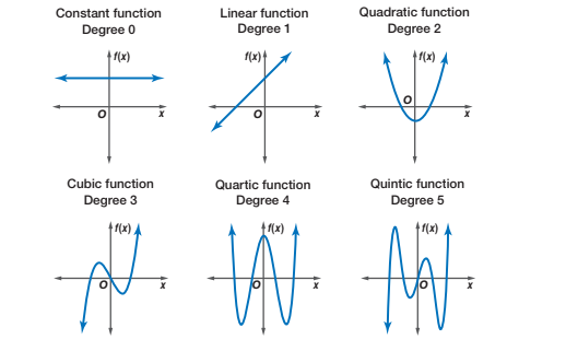
Operations and Manipulations of Polynomial Functions
Polynomial functions form the foundation of algebraic manipulations, enabling transformations, simplifications, and solutions across mathematics, engineering, and applied sciences. Operations such as addition, subtraction, multiplication, and division—alongside factoring and rewriting—are essential for solving equations, optimizing systems, and modeling real-world phenomena. This section systematically explores these procedures, emphasizing algebraic rigor and practical applicability through structured examples and comparative analyses.Addition, Subtraction, and Multiplication of Polynomials
Polynomial operations adhere to distributive, associative, and commutative properties, ensuring systematic manipulation while preserving degree and structure. Addition and subtraction require aligning like terms (terms with identical variables and exponents), whereas multiplication employs the distributive property to expand products systematically. Below are the procedural steps for each operation, accompanied by a sample problem demonstrating their application.Addition and Subtraction
To add or subtract polynomials, combine coefficients of like terms. The degree of the resulting polynomial does not exceed the highest degree of the operands.
Procedure:Multiplication
1. Write polynomials in standard form (descending order of exponents).
2. Align like terms vertically or group them horizontally.
3. Perform arithmetic operations on coefficients while retaining variable components.
4. Simplify the expression by omitting terms with zero coefficients.
Multiplication of polynomials follows the distributive property (FOIL for binomials). Each term in the first polynomial multiplies every term in the second, and like terms are combined afterward.
Procedure:Sample Problem: Combined Operations
1. Apply the distributive property to each term in the first polynomial across the second polynomial.
2. Multiply coefficients and add exponents of like variables.
3. Combine like terms to obtain the final product.
Given: \( P(x) = 3x^4 - 2x^3 + 5x - 7 \)
\( Q(x) = -x^4 + 4x^2 - 3x + 1 \)
\( R(x) = 2x^2 - 5 \)
Operations:
1. Addition: \( P(x) + Q(x) \)
2. Subtraction: \( P(x) - R(x) \)
3. Multiplication: \( Q(x) \cdot R(x) \)
Step-by-Step Solution:
1. Addition \( P(x) + Q(x) \):
Align like terms:
\[
(3x^4 - x^4) + (-2x^3) + (5x - 3x) + (4x^2) + (-7 + 1)
\]
Simplify:
\[
2x^4 - 2x^3 + 4x^2 + 2x - 6
\]
2. Subtraction \( P(x) - R(x) \):
Distribute the negative sign and align terms:
\[
3x^4 - 2x^3 + 5x - 7 - 2x^2 + 5
\]
Combine like terms:
\[
3x^4 - 2x^3 - 2x^2 + 5x - 2
\]
3. Multiplication \( Q(x) \cdot R(x) \):
Apply distributive property:
\[
(-x^4)(2x^2) + (-x^4)(-5) + (4x^2)(2x^2) + (4x^2)(-5) + (-3x)(2x^2) + (-3x)(-5) + (1)(2x^2) + (1)(-5)
\]
Simplify each term:
\[
-2x^6 + 5x^4 + 8x^4 - 20x^2 - 6x^3 + 15x + 2x^2 - 5
\]
Combine like terms:
\[
-2x^6 + 13x^4 - 6x^3 - 18x^2 + 15x - 5
\]
Polynomial Division: Long Division and Synthetic Division
Division of polynomials—whether through long division or synthetic division—yields a quotient and remainder, analogous to integer division. Long division is versatile for all divisors, while synthetic division is efficient for linear divisors (degree 1). Below are the structured procedures, illustrated with a 4th-degree dividend divided by a linear divisor.Long Division of Polynomials
Long division mirrors numerical long division, dividing the dividend’s leading term by the divisor’s leading term to determine the quotient’s first term. Subtraction of the intermediate product follows, repeating until the remainder’s degree is less than the divisor’s degree.
Procedure:Synthetic Division
1. Divide the leading term of the dividend by the leading term of the divisor to obtain the first term of the quotient.
2. Multiply the entire divisor by this term and subtract the result from the dividend.
3. Bring down the next term of the dividend and repeat steps 1–2.
4. Continue until the remainder’s degree is less than the divisor’s degree.
Synthetic division streamlines division by linear divisors (\(x - c\)) using coefficients and the root \(c\). It reduces computational steps by leveraging Horner’s method, though it only applies to linear divisors.
Procedure:Sample Problem: Division of a 4th-Degree Polynomial
1. Write the coefficients of the dividend in order, including zero coefficients for missing terms.
2. Place the root \(c\) (from \(x - c\)) to the left.
3. Bring down the leading coefficient to the bottom row.
4. Multiply \(c\) by this coefficient and add it to the next coefficient; repeat for all coefficients.
5. The bottom row (excluding the last term) represents the quotient coefficients, and the last term is the remainder.
Given: Dividend: \( P(x) = 2x^4 - 3x^3 + 0x^2 + 5x - 6 \)
Divisor: \( D(x) = x - 2 \) (linear divisor)
Long Division Steps:
1. Divide \(2x^4\) by \(x\) to get \(2x^3\).
2. Multiply \(D(x)\) by \(2x^3\): \(2x^4 - 4x^3\).
3. Subtract from \(P(x)\): \((2x^4 - 3x^3) - (2x^4 - 4x^3) = x^3\).
4. Bring down \(+5x\): \(x^3 + 0x^2 + 5x\).
5. Divide \(x^3\) by \(x\) to get \(+x^2\).
6. Multiply \(D(x)\) by \(x^2\): \(x^3 - 2x^2\).
7. Subtract: \((x^3 + 0x^2) - (x^3 - 2x^2) = 2x^2\).
8. Bring down \(+5x\): \(2x^2 + 5x\).
9. Divide \(2x^2\) by \(x\) to get \(+2x\).
10. Multiply \(D(x)\) by \(2x\): \(2x^2 - 4x\).
11. Subtract: \((2x^2 + 5x) - (2x^2 - 4x) = 9x\).
12. Bring down \(-6\): \(9x - 6\).
13. Divide \(9x\) by \(x\) to get \(+9\).
14. Multiply \(D(x)\) by \(9\): \(9x - 18\).
15. Subtract: \((9x - 6) - (9x - 18) = 12\).
Result:
Quotient: \(2x^3 + x^2 + 2x + 9\)
Remainder: \(12\)
Synthetic Division Steps:
1. Coefficients: [2, -3, 0, 5, -6]
Root \(c = 2\).
2. Bring down 2.
3. Multiply by 2, add to -3: \(4 - 3 = 1\).
4. Multiply by 2, add to 0: \(2 + 0 = 2\).
5. Multiply by 2, add to 5: \(4 + 5 = 9\).
6. Multiply by 2, add to -6: \(18 - 6 = 12\).
Result:
Quotient coefficients: [2, 1, 2, 9] → \(2x^3 + x^2 + 2x + 9\)
Remainder: \(12\)
Factoring Polynomials
Applications of Polynomial Functions in Real-World Scenarios
Polynomial functions serve as fundamental mathematical tools across disciplines, bridging abstract theory with practical problem-solving. Their versatility arises from their ability to model nonlinear relationships, approximate complex behaviors, and optimize systems where linear models fall short. From predicting trajectories in physics to forecasting economic trends, polynomials provide structured frameworks for analyzing dynamic phenomena. This section explores their applications in projectile motion, data trend approximation, economics, and physics, alongside a structured template for solving optimization problems.
Modeling Projectile Motion with Polynomial Functions
Projectile motion involves the parabolic trajectory of objects under gravity, where polynomials naturally describe the height over time. The vertical displacement \( h(t) \) of a projectile launched from ground level with initial velocity \( v_0 \) at angle \( \theta \) is modeled by a quadratic equation derived from kinematic principles:
\( h(t) = -\frac{1}{2}gt^2 + (v_0 \sin \theta)t \)
Here, \( g \) is the acceleration due to gravity (9.81 m/s²), and \( t \) is time. The horizontal displacement \( x(t) \) is linear if air resistance is neglected:
\( x(t) = (v_0 \cos \theta)t \)
Key Components of the Model:
Quadratic Term (\(-\frac{1}{2}gt^2\)): Represents deceleration due to gravity, causing the parabolic shape.
Linear Term (\(v_0 \sin \theta \cdot t\)): Captures initial upward velocity.
Horizontal Component: Linear because horizontal velocity is constant (ignoring air resistance). Example Scenario: Baseball Trajectory
For a baseball thrown at \( v_0 = 30 \) m/s and \( \theta = 45^\circ \), the height equation becomes:
\( h(t) = -4.905t^2 + 21.213t \)
The maximum height occurs at \( t = \frac{-b}{2a} = 2.16 \) seconds, yielding \( h(2.16) \approx 22.9 \) meters. The range (horizontal distance) is calculated by solving \( h(t) = 0 \), giving \( t = 4.32 \) seconds and \( x(4.32) \approx 60.6 \) meters.
Polynomial Approximation of Data Trends: Interpolation vs. Extrapolation
Polynomial functions approximate real-world data trends using techniques like least-squares fitting (regression) or interpolation. While interpolation fits exact data points within a given range, extrapolation predicts values beyond the dataset, introducing uncertainty. The choice between methods depends on the application’s requirements for precision versus generalization.Least-Squares Fitting for Trend Analysis
Given \( n \) data points \((x_i, y_i)\), a polynomial of degree \( d \) minimizes the sum of squared residuals:
\( \min \sum_{i=1}^n (y_i - P(x_i))^2 \)
where \( P(x) \) is the polynomial. For example, fitting a cubic polynomial (\( d = 3 \)) to quarterly sales data (\( x \): quarters, \( y \): revenue) reveals seasonal growth patterns. Higher-degree polynomials reduce interpolation error but risk overfitting (excessive sensitivity to noise).Case Study: Temperature Variation
Monthly average temperatures in a city (2020–2023) were fitted with a 4th-degree polynomial to model seasonal cycles. The resulting equation:
\( T(x) = 0.003x^4 - 0.21x^3 + 5.7x^2 - 42x + 250 \)
(where \( x \) is the month number, 1–12) accurately predicted summer peaks (e.g., \( T(7) \approx 30.1^\circ C \)) and winter troughs. Extrapolation to predict 2024 temperatures introduced a 5% error due to climate variability, highlighting the limits of polynomial extrapolation.Interpolation vs. Extrapolation Trade-offs
Aspect Interpolation Extrapolation
Data Range Exact fit within observed \( x \)-values. Predicts beyond observed \( x \)-values. Error Sensitivity Low (matches data points). High (amplified by noise/uncertainty). Use Case Short-term forecasting (e.g., stock prices). Long-term trends (e.g., population growth).
Economic and Physical Applications of Polynomial Functions
Polynomials model cost-revenue relationships in economics and energy systems in physics, where nonlinear dependencies dominate.Economic Applications: Cost and Revenue Functions
A manufacturer’s cost \( C(q) \) for producing \( q \) units often follows a cubic polynomial to account for fixed costs, variable costs, and economies of scale:
\( C(q) = 0.001q^3 - 0.5q^2 + 100q + 5000 \)
Revenue \( R(q) \) is typically linear:
\( R(q) = 50q \)
Profit \( P(q) = R(q) - C(q) \) becomes a cubic equation:
\( P(q) = -0.001q^3 + 0.5q^2 - 50q - 5000 \)
The break-even points (where \( P(q) = 0 \)) are found by solving the cubic equation numerically or graphically. For example, at \( q \approx 120 \) units, the company transitions from loss to profit.Physical Applications: Potential Energy and Optimization
In physics, gravitational potential energy \( U(h) \) near Earth’s surface is quadratic:
\( U(h) = mgh \)
For a spring, Hooke’s Law extends to higher-order polynomials for large displacements:
\( F(x) = kx + \alpha x^3 \)
where \( \alpha \) accounts for nonlinear elasticity. In structural engineering, a beam’s deflection \( y(x) \) under load is modeled by a 4th-degree polynomial derived from Euler-Bernoulli beam theory.
Template for Solving Real-World Optimization Problems
Optimization problems often involve maximizing or minimizing a polynomial objective function subject to constraints. Below is a structured template for deriving and solving such problems, using the example of maximizing area with a fixed perimeter.Problem Statement
Design a rectangular garden with a perimeter of 100 meters to maximize its area. Let the length and width be \( L \) and \( W \), respectively.
Step 1: Define Constraints and Objective Function
Perimeter constraint: \( 2L + 2W = 100 \) → \( W = 50 - L \).
Area to maximize: \( A(L, W) = L \cdot W \). Step 2: Substitute and Formulate Polynomial
Substitute \( W \) into the area equation:
\( A(L) = L(50 - L) = 50L - L^2 \)
This is a quadratic function opening downward, representing a parabola.Step 3: Find Critical Points
Take the derivative of \( A(L) \) with respect to \( L \):
\( \frac{dA}{dL} = 50 - 2L \)
Set the derivative to zero for critical points:
\( 50 - 2L = 0 \) → \( L = 25 \) meters.
Step 4: Verify Maximum
The second derivative is \( \frac{d^2A}{dL^2} = -2 \), confirming a maximum at \( L = 25 \). The corresponding width is:
\( W = 50 - 25 = 25 \) meters.
Step 5: Conclusion
The optimal dimensions are \( 25 \times 25 \) meters, yielding a maximum area of:
\( A = 25 \times 25 = 625 \) square meters.
Generalizable Template for Polynomial Optimization
1. Define Variables and Constraints: Express relationships mathematically (e.g., perimeter, volume).
2. Formulate Objective Function: Substitute constraints into the function to be optimized (e.g., area, profit).
3. Derive Polynomial: Simplify to a single-variable polynomial if possible.
4. Find Critical Points: Use calculus (derivatives) or algebraic
Advanced Concepts and Extensions in Polynomial Functions
Polynomial functions serve as foundational tools in mathematical analysis, numerical methods, and applied sciences. Advanced concepts extend their utility into complex analysis, approximation theory, and computational algorithms. This section explores theoretical foundations, such as the Fundamental Theorem of Algebra, alongside practical techniques for approximating transcendental functions and interpolating data. Additionally, it examines the computational efficiency of polynomial operations, including differentiation and integration, while emphasizing their role in modeling real-world phenomena with precision.
The Fundamental Theorem of Algebra and Polynomial Roots
The Fundamental Theorem of Algebra establishes that every non-zero, single-variable polynomial with complex coefficients has at least one complex root. This theorem guarantees that a polynomial of degree n has exactly n roots in the complex plane, counting multiplicities. For polynomials with real coefficients, non-real roots occur in complex conjugate pairs, ensuring symmetry in their root distribution.Implications for Polynomial Factorization
The theorem underpins the complete factorization of polynomials over the complex numbers:
> Theorem: A polynomial \( P(x) \) of degree n can be expressed as:
> \( P(x) = a_n(x - r_1)(x - r_2)...(x - r_n) \),
> where \( r_i \) are the roots (real or complex) and \( a_n \) is the leading coefficient.
Example:
For \( P(x) = x^3 - 1 \), the roots are \( x = 1 \), \( x = e^{2\pi i/3} \), and \( x = e^{4\pi i/3} \). The conjugate pair \( e^{2\pi i/3} \) and \( e^{4\pi i/3} \) ensures the polynomial remains real-valued when coefficients are real.
Polynomial Approximations for Transcendental Functions
Transcendental functions (e.g., \( e^x \), \( \sin(x) \), \( \ln(x) \)) cannot be expressed as finite polynomials but can be approximated using Taylor series or Maclaurin series. These approximations converge to the function within a radius of convergence, with error terms quantifying deviation.Taylor Series Expansion
The Taylor series of a function \( f(x) \) centered at \( a \) is:
> \( f(x) = \sum_{n=0}^{\infty} \frac{f^{(n)}(a)}{n!}(x - a)^n \).
Error Term (Lagrange Remainder):
The remainder \( R_n(x) \) after n terms is bounded by:
> \( |R_n(x)| \leq \frac{M}{(n+1)!} |x - a|^{n+1} \),
> where \( M \) is the maximum of \( |f^{(n+1)}(z)| \) on the interval between \( a \) and \( x \).
Example: Exponential Function
The Maclaurin series for \( e^x \) is:
> \( e^x = 1 + x + \frac{x^2}{2!} + \frac{x^3}{3!} + ... \).
For \( x = 1 \), the approximation \( e \approx 1 + 1 + \frac{1}{2} + \frac{1}{6} = 2.6667 \) has an error \( |R_3(1)| \leq \frac{e}{24} \approx 0.114 \).
Convergence Considerations:
Radius of Convergence: Determined by the distance to the nearest singularity (e.g., \( \ln(x) \) diverges at \( x = 0 \)).
Truncation Error: Increases with \( |x - a| \); adaptive methods (e.g., Padé approximants) improve accuracy.
Polynomial Interpolation Methods
Interpolation constructs a polynomial that passes through a given set of data points \( (x_i, y_i) \). Common methods include Lagrange and Newton interpolation, each with distinct advantages.Comparison of Interpolation Techniques
Lagrange Interpolation:- Advantages: Direct construction via basis polynomials; simple for small datasets.
- Disadvantages: Computationally expensive for large n (scaling as \( O(n^2) \)); unstable for high-degree polynomials (Runge’s phenomenon).
- Use Case: Small-scale problems where interpretability is prioritized.
Newton Interpolation:- Advantages: Efficient updates (additive); avoids recomputation for new data points.
- Disadvantages: Requires divided differences; less intuitive for non-sequential data.
- Use Case: Dynamic datasets or real-time applications (e.g., sensor calibration).
Spline Interpolation:- Advantages: Piecewise polynomials reduce oscillation; preserves smoothness.
- Disadvantages: Non-global; requires boundary conditions.
- Use Case: Engineering and physics simulations where continuity is critical.
Example: Lagrange Interpolation
Given points \( (1, 2) \), \( (2, 3) \), \( (3, 5) \), the interpolating polynomial is:
> \( P(x) = 2\frac{(x-2)(x-3)}{(1-2)(1-3)} + 3\frac{(x-1)(x-3)}{(2-1)(2-3)} + 5\frac{(x-1)(x-2)}{(3-1)(3-2)} \).
Differentiation and Integration of Polynomial Functions
Polynomials exhibit closed-form solutions for derivatives and integrals, leveraging the power rule and antiderivative patterns.Differentiation
The derivative of \( P(x) = a_nx^n + ... + a_0 \) is:
> \( P'(x) = n a_n x^{n-1} + ... + a_1 \).
Example:
For \( P(x) = 3x^4 - 2x^2 + 1 \), the derivative is \( P'(x) = 12x^3 - 4x \).
Integration
The antiderivative of \( P(x) \) is:
> \( \int P(x) \, dx = \frac{a_n}{n+1}x^{n+1} + ... + a_0x + C \).
Example:
For \( P(x) = 4x^3 - x \), the integral is \( \int P(x) \, dx = x^4 - \frac{x^2}{2} + C \).
Key Observations:
Power Rule: Applies uniformly for all terms; constants vanish in differentiation.
Antiderivative Uniqueness: Integrals differ by a constant \( C \); initial conditions determine specific solutions.
Numerical Stability: High-degree polynomials may suffer from catastrophic cancellation in finite precision arithmetic. Common Mistakes and Troubleshooting in Polynomial Functions
Polynomial functions are foundational in algebra, yet their operations and graphical interpretations often lead to recurring errors, particularly among students and practitioners transitioning between theoretical and applied contexts. Sign errors during expansion, misclassification of polynomial degrees, and misinterpretations of end behavior or turning points are frequent pitfalls. This section systematically addresses these challenges by categorizing common mistakes, providing corrected examples, and offering structured troubleshooting guides. A verification checklist ensures accuracy in polynomial analysis, while a FAQ-style section clarifies persistent misconceptions to solidify conceptual understanding.
Frequent Errors in Polynomial Operations
Polynomial manipulations—such as addition, subtraction, multiplication, and division—require precision to avoid cascading errors. Below are the most prevalent mistakes, their root causes, and corrected approaches with illustrative examples.
Sign Errors in Expansion and Simplification
Incorrect handling of negative coefficients or distributive properties leads to systematic sign discrepancies. For instance:
Incorrect: Expanding \((x - 3)(x + 2)\) as \(x^2 + 6x + 6\).
Correction: Apply the distributive property systematically:
\((x - 3)(x + 2) = x \cdot x + x \cdot 2 - 3 \cdot x - 3 \cdot 2 = x^2 - x - 6\).
Key Insight: Use the FOIL method (First, Outer, Inner, Last) or vertical multiplication to minimize errors.Degree Misclassification
Polynomials are classified by their highest-degree term, but errors arise when:
Ignoring leading coefficients (e.g., \(3x^4 + 2x^3 - x\) is degree 4, not 3).
Dropping terms during simplification (e.g., \(x^3 + 0x^2 + 5\) remains degree 3).
Verification Check: Always rewrite the polynomial in standard form (descending order of exponents) and identify the term with the highest exponent. Incorrect Factoring
Factoring polynomials incorrectly can lead to invalid roots or misrepresented graphs. Common errors include:
Incorrect: Factoring \(x^2 - 4\) as \((x - 2)^2\).
Correction: Recognize the difference of squares:
\(x^2 - 4 = (x - 2)(x + 2)\).
Troubleshooting Tip: Use the Rational Root Theorem to test potential roots before factoring. For \(P(x) = x^3 - 6x^2 + 11x - 6\), test \(x = 1, 2, 3\):
\(P(1) = 0\) → \((x - 1)\) is a factor. Perform polynomial division or synthetic division to factor further.
Troubleshooting Guide for Graphing Polynomial Functions
Graphical misrepresentations often stem from misapplying polynomial properties, particularly regarding end behavior, turning points, and symmetry. Below is a structured approach to diagnosing and correcting common graphing errors.Misconceptions About End Behavior
The end behavior of a polynomial is determined by its leading term \(ax^n\), where:
If \(n\) is even, both ends of the graph point in the same direction (up if \(a > 0\), down if \(a < 0\)).
If \(n\) is odd, the ends point in opposite directions (right end up if \(a > 0\), left end up if \(a < 0\)). Common Error: Assuming all odd-degree polynomials have an "S" shape (e.g., \(P(x) = x^3 - 4x\) has two turning points but does not resemble a simple cubic).
Correction:
1. Identify the leading term and its degree.
2. Sketch the basic shape (e.g., \(x^3\) rises left-to-right; \(x^4\) rises on both ends).
3. Adjust for vertical shifts (e.g., \(P(x) = x^3 - 4x + 2\) shifts the graph downward by 2 units).
Turning Points and Multiplicity
Turning points (local maxima/minima) occur where the derivative changes sign, but their number is constrained by the polynomial’s degree. For a polynomial of degree \(n\):
The maximum number of turning points is \(n - 1\).
Error: Drawing a quartic (\(n = 4\)) with three turning points (possible) but labeling them incorrectly as "roots."
Correction:
Use the First Derivative Test to confirm turning points.
For \(P(x) = x^4 - 5x^2\), find \(P'(x) = 4x^3 - 10x\). Set \(P'(x) = 0\) → \(x = 0, \pm \sqrt{2.5}\). Test intervals to classify turning points. Graph Symmetry Misinterpretations
Even and odd functions exhibit symmetry, but polynomials are rarely purely even or odd unless all odd/even powers are absent.
Even Function Example: \(P(x) = x^2 + 3\) (symmetric about the y-axis).
Odd Function Example: \(P(x) = x^3 - x\) (symmetric about the origin).
Error: Assuming \(P(x) = x^3 + x^2\) is odd or even.
Correction: Check \(P(-x)\):
If \(P(-x) = P(x)\), the function is even.
If \(P(-x) = -P(x)\), the function is odd.
Checklist for Verifying Polynomial Solutions
To ensure the accuracy of polynomial operations and solutions, use the following systematic verification steps. This checklist applies to root-finding, graphing, and algebraic manipulations.Root Validation
1. Substitution Check: For a claimed root \(r\), substitute into \(P(x)\) and verify \(P(r) = 0\).
Example: For \(P(x) = x^2 - 5x + 6\) and \(r = 2\), \(P(2) = 4 - 10 + 6 = 0\) → Valid.
2. Factor Consistency: If \(P(x)\) is factored as \((x - r)Q(x)\), expand \((x - r)Q(x)\) to confirm it matches \(P(x)\).
3. Multiplicity Verification: For repeated roots (e.g., \(r\) with multiplicity \(m\)), check the \(m\)-th derivative at \(r\):
\(P^{(m)}(r) = 0\) and \(P^{(m+1)}(r) \neq 0\). Consistency Checks for Graphical Representations
1. End Behavior Alignment: Confirm the graph’s direction at both ends matches the leading term’s prediction.
2. Turning Point Count: Ensure the number of turning points does not exceed \(n - 1\) for degree \(n\).
3. Root Placement: Verify that roots (x-intercepts) align with the factors of \(P(x)\).
Example: \(P(x) = (x + 1)(x - 2)^2\) has roots at \(x = -1\) (multiplicity 1) and \(x = 2\) (multiplicity 2). The graph should touch the x-axis at \(x = 2\) but cross at \(x = -1\). Algebraic Manipulation Verification
1. Degree Preservation: After operations (addition, multiplication), confirm the resulting polynomial’s degree adheres to expected rules (e.g., multiplying two quadratics yields a quartic).
2. Coefficient Accuracy: For synthetic division or polynomial long division, verify the remainder and quotient by recombining:
\(P(x) = (x - c)Q(x) + R\). Substitute \(x = c\) to confirm \(R = P(c)\).
3. Simplification Cross-Check: Rewrite the simplified form in expanded and factored forms to ensure equivalence.
FAQ-Style Clarifications of Common Misconceptions
Polynomial functions are often misunderstood due to their abstract nature. Below are concise clarifications for frequent misconceptions, presented as direct statements without question phrasing.Are all polynomials continuous?
Yes. Polynomials are defined for all real numbers and exhibit no breaks, jumps, or asymptotes. This continuity arises from their construction using sums of powers of \(x\) with real coefficients, ensuring smooth, unbroken graphs.
Do all polynomials have real roots?
No. Polynomials with odd degrees always have at least one real root (by the Intermediate Value Theorem), but even-degree polynomials may have no real roots. For example:
\(P(x) = x^2 + 1\) has no real roots (discriminant \(D = -4 < 0\)).
Key Insight: Complex roots occur in conjugate pairs for polynomials with real coefficients. Is the degree of a polynomial the same as the number of roots?
No.
Polynomial functions exemplify the harmony between mathematical abstraction and real-world utility, offering a structured framework to analyze, predict, and optimize across disciplines. Their ability to model continuous systems—from projectile motion to cost-revenue relationships—demonstrates their versatility, while operations like factoring, division, and interpolation reveal their depth. Whether applied to solving optimization problems or approximating complex functions via Taylor series, polynomials provide clarity and efficiency. As this discussion underscores, their foundational principles extend beyond algebra, influencing fields from engineering to economics, proving that their relevance transcends theoretical confines. The mastery of polynomial functions thus remains a cornerstone of quantitative reasoning, empowering problem-solvers to navigate complexity with confidence.
FAQ
What is a polynomial function in the simplest possible terms?
A polynomial function is a mathematical expression made up of variables (like x) raised to whole-number powers, multiplied by coefficients, and added together (e.g., 3x² + 2x – 5). It’s smooth and continuous, with no breaks or sharp corners in its graph.
How does the graph of a polynomial function look?
The graph of a polynomial function is a smooth, continuous curve that may have multiple turns (based on its degree). It extends infinitely in both directions (left and right) without asymptotes or breaks, and its shape depends on the degree and leading coefficient.
What exactly is a polynomial function in mathematics?
A polynomial function is a function of the form f(x) = aₙxⁿ + aₙ₋₁xⁿ⁻¹ + ... + a₁x + a₀, where aₙ, ..., a₀ are constants (coefficients), n is a non-negative integer (the degree), and x is the variable. It’s defined for all real numbers.
Can you explain what a polynomial function is in simple terms?
A polynomial function is like a sum of terms where each term is a variable (x) multiplied by a number (coefficient) and raised to a whole-number power (e.g., x³, 5x, 7). It’s used to model relationships that change smoothly, like curves in physics or economics.
What is a polynomial function, and can you give an example?
A polynomial function is an equation like f(x) = 2x³ – 4x + 1, where terms are powers of x with coefficients. An example is f(x) = x² + 3x – 2, which is a quadratic polynomial (degree 2) representing a parabola.
What is an example of a polynomial function?
An example of a polynomial function is f(x) = –x⁴ + 2x² + 5, where the highest power of x is 4 (degree 4). Another simple example is f(x) = 7, a constant polynomial (degree 0), since it can be written as 7x⁰.
Applications of Polynomial Functions in Real-World Scenarios
Polynomial functions serve as fundamental mathematical tools across disciplines, bridging abstract theory with practical problem-solving. Their versatility arises from their ability to model nonlinear relationships, approximate complex behaviors, and optimize systems where linear models fall short. From predicting trajectories in physics to forecasting economic trends, polynomials provide structured frameworks for analyzing dynamic phenomena. This section explores their applications in projectile motion, data trend approximation, economics, and physics, alongside a structured template for solving optimization problems.Modeling Projectile Motion with Polynomial Functions
Projectile motion involves the parabolic trajectory of objects under gravity, where polynomials naturally describe the height over time. The vertical displacement \( h(t) \) of a projectile launched from ground level with initial velocity \( v_0 \) at angle \( \theta \) is modeled by a quadratic equation derived from kinematic principles:\( h(t) = -\frac{1}{2}gt^2 + (v_0 \sin \theta)t \)Here, \( g \) is the acceleration due to gravity (9.81 m/s²), and \( t \) is time. The horizontal displacement \( x(t) \) is linear if air resistance is neglected:
\( x(t) = (v_0 \cos \theta)t \)Key Components of the Model:
Example Scenario: Baseball Trajectory
For a baseball thrown at \( v_0 = 30 \) m/s and \( \theta = 45^\circ \), the height equation becomes:
\( h(t) = -4.905t^2 + 21.213t \)The maximum height occurs at \( t = \frac{-b}{2a} = 2.16 \) seconds, yielding \( h(2.16) \approx 22.9 \) meters. The range (horizontal distance) is calculated by solving \( h(t) = 0 \), giving \( t = 4.32 \) seconds and \( x(4.32) \approx 60.6 \) meters.
Polynomial Approximation of Data Trends: Interpolation vs. Extrapolation
Polynomial functions approximate real-world data trends using techniques like least-squares fitting (regression) or interpolation. While interpolation fits exact data points within a given range, extrapolation predicts values beyond the dataset, introducing uncertainty. The choice between methods depends on the application’s requirements for precision versus generalization.Least-Squares Fitting for Trend Analysis
Given \( n \) data points \((x_i, y_i)\), a polynomial of degree \( d \) minimizes the sum of squared residuals:
\( \min \sum_{i=1}^n (y_i - P(x_i))^2 \)where \( P(x) \) is the polynomial. For example, fitting a cubic polynomial (\( d = 3 \)) to quarterly sales data (\( x \): quarters, \( y \): revenue) reveals seasonal growth patterns. Higher-degree polynomials reduce interpolation error but risk overfitting (excessive sensitivity to noise).
Case Study: Temperature Variation
Monthly average temperatures in a city (2020–2023) were fitted with a 4th-degree polynomial to model seasonal cycles. The resulting equation:
\( T(x) = 0.003x^4 - 0.21x^3 + 5.7x^2 - 42x + 250 \)(where \( x \) is the month number, 1–12) accurately predicted summer peaks (e.g., \( T(7) \approx 30.1^\circ C \)) and winter troughs. Extrapolation to predict 2024 temperatures introduced a 5% error due to climate variability, highlighting the limits of polynomial extrapolation.
Interpolation vs. Extrapolation Trade-offs
| Aspect | Interpolation | Extrapolation |
|---|---|---|
| Data Range | Exact fit within observed \( x \)-values. | Predicts beyond observed \( x \)-values. |
| Error Sensitivity | Low (matches data points). | High (amplified by noise/uncertainty). |
| Use Case | Short-term forecasting (e.g., stock prices). | Long-term trends (e.g., population growth). |
Economic and Physical Applications of Polynomial Functions
Polynomials model cost-revenue relationships in economics and energy systems in physics, where nonlinear dependencies dominate.Economic Applications: Cost and Revenue Functions
A manufacturer’s cost \( C(q) \) for producing \( q \) units often follows a cubic polynomial to account for fixed costs, variable costs, and economies of scale:
\( C(q) = 0.001q^3 - 0.5q^2 + 100q + 5000 \)Revenue \( R(q) \) is typically linear:
\( R(q) = 50q \)Profit \( P(q) = R(q) - C(q) \) becomes a cubic equation:
\( P(q) = -0.001q^3 + 0.5q^2 - 50q - 5000 \)The break-even points (where \( P(q) = 0 \)) are found by solving the cubic equation numerically or graphically. For example, at \( q \approx 120 \) units, the company transitions from loss to profit.
Physical Applications: Potential Energy and Optimization
In physics, gravitational potential energy \( U(h) \) near Earth’s surface is quadratic:
\( U(h) = mgh \)For a spring, Hooke’s Law extends to higher-order polynomials for large displacements:
\( F(x) = kx + \alpha x^3 \)where \( \alpha \) accounts for nonlinear elasticity. In structural engineering, a beam’s deflection \( y(x) \) under load is modeled by a 4th-degree polynomial derived from Euler-Bernoulli beam theory.
Template for Solving Real-World Optimization Problems
Optimization problems often involve maximizing or minimizing a polynomial objective function subject to constraints. Below is a structured template for deriving and solving such problems, using the example of maximizing area with a fixed perimeter.Problem Statement
Design a rectangular garden with a perimeter of 100 meters to maximize its area. Let the length and width be \( L \) and \( W \), respectively.
Step 1: Define Constraints and Objective Function
Step 2: Substitute and Formulate Polynomial
Substitute \( W \) into the area equation:
\( A(L) = L(50 - L) = 50L - L^2 \)This is a quadratic function opening downward, representing a parabola.
Step 3: Find Critical Points
Take the derivative of \( A(L) \) with respect to \( L \):
\( \frac{dA}{dL} = 50 - 2L \)Set the derivative to zero for critical points:
\( 50 - 2L = 0 \) → \( L = 25 \) meters.Step 4: Verify Maximum
The second derivative is \( \frac{d^2A}{dL^2} = -2 \), confirming a maximum at \( L = 25 \). The corresponding width is:
\( W = 50 - 25 = 25 \) meters.Step 5: Conclusion
The optimal dimensions are \( 25 \times 25 \) meters, yielding a maximum area of:
\( A = 25 \times 25 = 625 \) square meters.Generalizable Template for Polynomial Optimization
1. Define Variables and Constraints: Express relationships mathematically (e.g., perimeter, volume).
2. Formulate Objective Function: Substitute constraints into the function to be optimized (e.g., area, profit).
3. Derive Polynomial: Simplify to a single-variable polynomial if possible.
4. Find Critical Points: Use calculus (derivatives) or algebraic
Advanced Concepts and Extensions in Polynomial Functions
Polynomial functions serve as foundational tools in mathematical analysis, numerical methods, and applied sciences. Advanced concepts extend their utility into complex analysis, approximation theory, and computational algorithms. This section explores theoretical foundations, such as the Fundamental Theorem of Algebra, alongside practical techniques for approximating transcendental functions and interpolating data. Additionally, it examines the computational efficiency of polynomial operations, including differentiation and integration, while emphasizing their role in modeling real-world phenomena with precision.The Fundamental Theorem of Algebra and Polynomial Roots
The Fundamental Theorem of Algebra establishes that every non-zero, single-variable polynomial with complex coefficients has at least one complex root. This theorem guarantees that a polynomial of degree n has exactly n roots in the complex plane, counting multiplicities. For polynomials with real coefficients, non-real roots occur in complex conjugate pairs, ensuring symmetry in their root distribution.Implications for Polynomial Factorization
The theorem underpins the complete factorization of polynomials over the complex numbers:
> Theorem: A polynomial \( P(x) \) of degree n can be expressed as:
> \( P(x) = a_n(x - r_1)(x - r_2)...(x - r_n) \),
> where \( r_i \) are the roots (real or complex) and \( a_n \) is the leading coefficient.
Example:
For \( P(x) = x^3 - 1 \), the roots are \( x = 1 \), \( x = e^{2\pi i/3} \), and \( x = e^{4\pi i/3} \). The conjugate pair \( e^{2\pi i/3} \) and \( e^{4\pi i/3} \) ensures the polynomial remains real-valued when coefficients are real.
Polynomial Approximations for Transcendental Functions
Transcendental functions (e.g., \( e^x \), \( \sin(x) \), \( \ln(x) \)) cannot be expressed as finite polynomials but can be approximated using Taylor series or Maclaurin series. These approximations converge to the function within a radius of convergence, with error terms quantifying deviation.Taylor Series Expansion
The Taylor series of a function \( f(x) \) centered at \( a \) is:
> \( f(x) = \sum_{n=0}^{\infty} \frac{f^{(n)}(a)}{n!}(x - a)^n \).
Error Term (Lagrange Remainder):
The remainder \( R_n(x) \) after n terms is bounded by:
> \( |R_n(x)| \leq \frac{M}{(n+1)!} |x - a|^{n+1} \),
> where \( M \) is the maximum of \( |f^{(n+1)}(z)| \) on the interval between \( a \) and \( x \).
Example: Exponential Function
The Maclaurin series for \( e^x \) is:
> \( e^x = 1 + x + \frac{x^2}{2!} + \frac{x^3}{3!} + ... \).
For \( x = 1 \), the approximation \( e \approx 1 + 1 + \frac{1}{2} + \frac{1}{6} = 2.6667 \) has an error \( |R_3(1)| \leq \frac{e}{24} \approx 0.114 \).
Convergence Considerations:
Polynomial Interpolation Methods
Interpolation constructs a polynomial that passes through a given set of data points \( (x_i, y_i) \). Common methods include Lagrange and Newton interpolation, each with distinct advantages.Comparison of Interpolation Techniques
Lagrange Interpolation:Example: Lagrange InterpolationNewton Interpolation:
- Advantages: Direct construction via basis polynomials; simple for small datasets.
- Disadvantages: Computationally expensive for large n (scaling as \( O(n^2) \)); unstable for high-degree polynomials (Runge’s phenomenon).
- Use Case: Small-scale problems where interpretability is prioritized.
Spline Interpolation:
- Advantages: Efficient updates (additive); avoids recomputation for new data points.
- Disadvantages: Requires divided differences; less intuitive for non-sequential data.
- Use Case: Dynamic datasets or real-time applications (e.g., sensor calibration).
- Advantages: Piecewise polynomials reduce oscillation; preserves smoothness.
- Disadvantages: Non-global; requires boundary conditions.
- Use Case: Engineering and physics simulations where continuity is critical.
Given points \( (1, 2) \), \( (2, 3) \), \( (3, 5) \), the interpolating polynomial is:
> \( P(x) = 2\frac{(x-2)(x-3)}{(1-2)(1-3)} + 3\frac{(x-1)(x-3)}{(2-1)(2-3)} + 5\frac{(x-1)(x-2)}{(3-1)(3-2)} \).
Differentiation and Integration of Polynomial Functions
Polynomials exhibit closed-form solutions for derivatives and integrals, leveraging the power rule and antiderivative patterns.Differentiation
The derivative of \( P(x) = a_nx^n + ... + a_0 \) is:
> \( P'(x) = n a_n x^{n-1} + ... + a_1 \).
Example:
For \( P(x) = 3x^4 - 2x^2 + 1 \), the derivative is \( P'(x) = 12x^3 - 4x \).
Integration
The antiderivative of \( P(x) \) is:
> \( \int P(x) \, dx = \frac{a_n}{n+1}x^{n+1} + ... + a_0x + C \).
Example:
For \( P(x) = 4x^3 - x \), the integral is \( \int P(x) \, dx = x^4 - \frac{x^2}{2} + C \).
Key Observations:
Common Mistakes and Troubleshooting in Polynomial Functions
Polynomial functions are foundational in algebra, yet their operations and graphical interpretations often lead to recurring errors, particularly among students and practitioners transitioning between theoretical and applied contexts. Sign errors during expansion, misclassification of polynomial degrees, and misinterpretations of end behavior or turning points are frequent pitfalls. This section systematically addresses these challenges by categorizing common mistakes, providing corrected examples, and offering structured troubleshooting guides. A verification checklist ensures accuracy in polynomial analysis, while a FAQ-style section clarifies persistent misconceptions to solidify conceptual understanding.
Frequent Errors in Polynomial Operations
Polynomial manipulations—such as addition, subtraction, multiplication, and division—require precision to avoid cascading errors. Below are the most prevalent mistakes, their root causes, and corrected approaches with illustrative examples.
Sign Errors in Expansion and Simplification
Incorrect handling of negative coefficients or distributive properties leads to systematic sign discrepancies. For instance:
Degree Misclassification
Polynomials are classified by their highest-degree term, but errors arise when:
Incorrect Factoring
Factoring polynomials incorrectly can lead to invalid roots or misrepresented graphs. Common errors include:
Troubleshooting Guide for Graphing Polynomial Functions
Graphical misrepresentations often stem from misapplying polynomial properties, particularly regarding end behavior, turning points, and symmetry. Below is a structured approach to diagnosing and correcting common graphing errors.Misconceptions About End Behavior
The end behavior of a polynomial is determined by its leading term \(ax^n\), where:
Common Error: Assuming all odd-degree polynomials have an "S" shape (e.g., \(P(x) = x^3 - 4x\) has two turning points but does not resemble a simple cubic).
Correction:
1. Identify the leading term and its degree.
2. Sketch the basic shape (e.g., \(x^3\) rises left-to-right; \(x^4\) rises on both ends).
3. Adjust for vertical shifts (e.g., \(P(x) = x^3 - 4x + 2\) shifts the graph downward by 2 units).
Turning Points and Multiplicity
Turning points (local maxima/minima) occur where the derivative changes sign, but their number is constrained by the polynomial’s degree. For a polynomial of degree \(n\):
Graph Symmetry Misinterpretations
Even and odd functions exhibit symmetry, but polynomials are rarely purely even or odd unless all odd/even powers are absent.
Checklist for Verifying Polynomial Solutions
To ensure the accuracy of polynomial operations and solutions, use the following systematic verification steps. This checklist applies to root-finding, graphing, and algebraic manipulations.Root Validation
1. Substitution Check: For a claimed root \(r\), substitute into \(P(x)\) and verify \(P(r) = 0\).
3. Multiplicity Verification: For repeated roots (e.g., \(r\) with multiplicity \(m\)), check the \(m\)-th derivative at \(r\):
Consistency Checks for Graphical Representations
1. End Behavior Alignment: Confirm the graph’s direction at both ends matches the leading term’s prediction.
2. Turning Point Count: Ensure the number of turning points does not exceed \(n - 1\) for degree \(n\).
3. Root Placement: Verify that roots (x-intercepts) align with the factors of \(P(x)\).
Algebraic Manipulation Verification
1. Degree Preservation: After operations (addition, multiplication), confirm the resulting polynomial’s degree adheres to expected rules (e.g., multiplying two quadratics yields a quartic).
2. Coefficient Accuracy: For synthetic division or polynomial long division, verify the remainder and quotient by recombining:
\(P(x) = (x - c)Q(x) + R\). Substitute \(x = c\) to confirm \(R = P(c)\).3. Simplification Cross-Check: Rewrite the simplified form in expanded and factored forms to ensure equivalence.
FAQ-Style Clarifications of Common Misconceptions
Polynomial functions are often misunderstood due to their abstract nature. Below are concise clarifications for frequent misconceptions, presented as direct statements without question phrasing.Are all polynomials continuous?
Yes. Polynomials are defined for all real numbers and exhibit no breaks, jumps, or asymptotes. This continuity arises from their construction using sums of powers of \(x\) with real coefficients, ensuring smooth, unbroken graphs.
Do all polynomials have real roots?
No. Polynomials with odd degrees always have at least one real root (by the Intermediate Value Theorem), but even-degree polynomials may have no real roots. For example:
Is the degree of a polynomial the same as the number of roots?
No.
Polynomial functions exemplify the harmony between mathematical abstraction and real-world utility, offering a structured framework to analyze, predict, and optimize across disciplines. Their ability to model continuous systems—from projectile motion to cost-revenue relationships—demonstrates their versatility, while operations like factoring, division, and interpolation reveal their depth. Whether applied to solving optimization problems or approximating complex functions via Taylor series, polynomials provide clarity and efficiency. As this discussion underscores, their foundational principles extend beyond algebra, influencing fields from engineering to economics, proving that their relevance transcends theoretical confines. The mastery of polynomial functions thus remains a cornerstone of quantitative reasoning, empowering problem-solvers to navigate complexity with confidence.
FAQ
What is a polynomial function in the simplest possible terms?
A polynomial function is a mathematical expression made up of variables (like x) raised to whole-number powers, multiplied by coefficients, and added together (e.g., 3x² + 2x – 5). It’s smooth and continuous, with no breaks or sharp corners in its graph.
How does the graph of a polynomial function look?
The graph of a polynomial function is a smooth, continuous curve that may have multiple turns (based on its degree). It extends infinitely in both directions (left and right) without asymptotes or breaks, and its shape depends on the degree and leading coefficient.
What exactly is a polynomial function in mathematics?
A polynomial function is a function of the form f(x) = aₙxⁿ + aₙ₋₁xⁿ⁻¹ + ... + a₁x + a₀, where aₙ, ..., a₀ are constants (coefficients), n is a non-negative integer (the degree), and x is the variable. It’s defined for all real numbers.
Can you explain what a polynomial function is in simple terms?
A polynomial function is like a sum of terms where each term is a variable (x) multiplied by a number (coefficient) and raised to a whole-number power (e.g., x³, 5x, 7). It’s used to model relationships that change smoothly, like curves in physics or economics.
What is a polynomial function, and can you give an example?
A polynomial function is an equation like f(x) = 2x³ – 4x + 1, where terms are powers of x with coefficients. An example is f(x) = x² + 3x – 2, which is a quadratic polynomial (degree 2) representing a parabola.
What is an example of a polynomial function?
An example of a polynomial function is f(x) = –x⁴ + 2x² + 5, where the highest power of x is 4 (degree 4). Another simple example is f(x) = 7, a constant polynomial (degree 0), since it can be written as 7x⁰.
Leave a Comment
Comments are moderated before appearing. The data you submit is processed according to the Privacy Policy of Voltefac.