What Is Observability Fundamentals Structure And Impact
Table of Contents
- Core Definition and Evolution of Observability
- Foundational Principles of Observability
- Historical Progression and Key Milestones
- Comparative Analysis: Observability vs. Monitoring vs. Logging
- Influential Frameworks and Methodologies
- Core Tenet of Observability
- Three Pillars of Observability: Metrics, Logs, and Traces
- Metrics: Quantifying System Health with Time-Series Data
- Logs: Structured and Unstructured Event Records for Debugging
- Distributed Traces: Mapping Request Flows Across Microservices
- Comparison of Observability Pillars: Metrics, Logs, and Traces
- Observability in Distributed Systems and Microservices
- Challenges in Distributed Architectures and Observability Requirements
- Context Propagation and the W3C Trace Context Standard
- Sampling Strategies for Traces in High-Throughput Systems
- Decision Flowchart for Selecting Observability Tools by System Complexity
- Tools and Technologies for Implementing Observability
- Comparison of Open-Source and Commercial Observability Platforms
- Essential Components of a Modern Observability Stack
- Configuring Prometheus for a Node.js Application
- Grafana Dashboard Template for SLOs and Error Budgets
- Role of AIOps in Augmenting Observability
- FAQ
- what is observability in software?
- what is observability in ai?
- what is observability in devops?
- what is observability in agentic ai?
- what is observability and monitoring?
- what is observability in tech?
Observability represents a paradigm shift in how modern software systems are understood, operated, and optimized—moving beyond traditional reactive monitoring to proactive, data-driven insights. Unlike legacy approaches that merely track predefined metrics or log events, observability enables teams to infer system behavior dynamically, diagnosing issues before they escalate into outages. Rooted in distributed architectures and reinforced by frameworks like Google’s Site Reliability Engineering (SRE) and Netflix’s chaos engineering, this discipline has evolved from static alerts into a continuous feedback loop that aligns technical performance with business objectives.
The core principle hinges on collecting, correlating, and contextualizing three critical data streams: metrics, logs, and traces. While metrics quantify system health (e.g., latency, throughput), logs provide granular debugging context, and traces map request flows across microservices, exposing hidden dependencies. This trifecta transforms reactive troubleshooting into predictive resilience, particularly in environments where complexity—such as Kubernetes clusters or serverless functions—obscures root causes. By bridging gaps left by conventional monitoring, observability empowers engineers to ask why a system fails, not just what failed, thereby reducing mean time to resolution (MTTR) and improving system reliability.
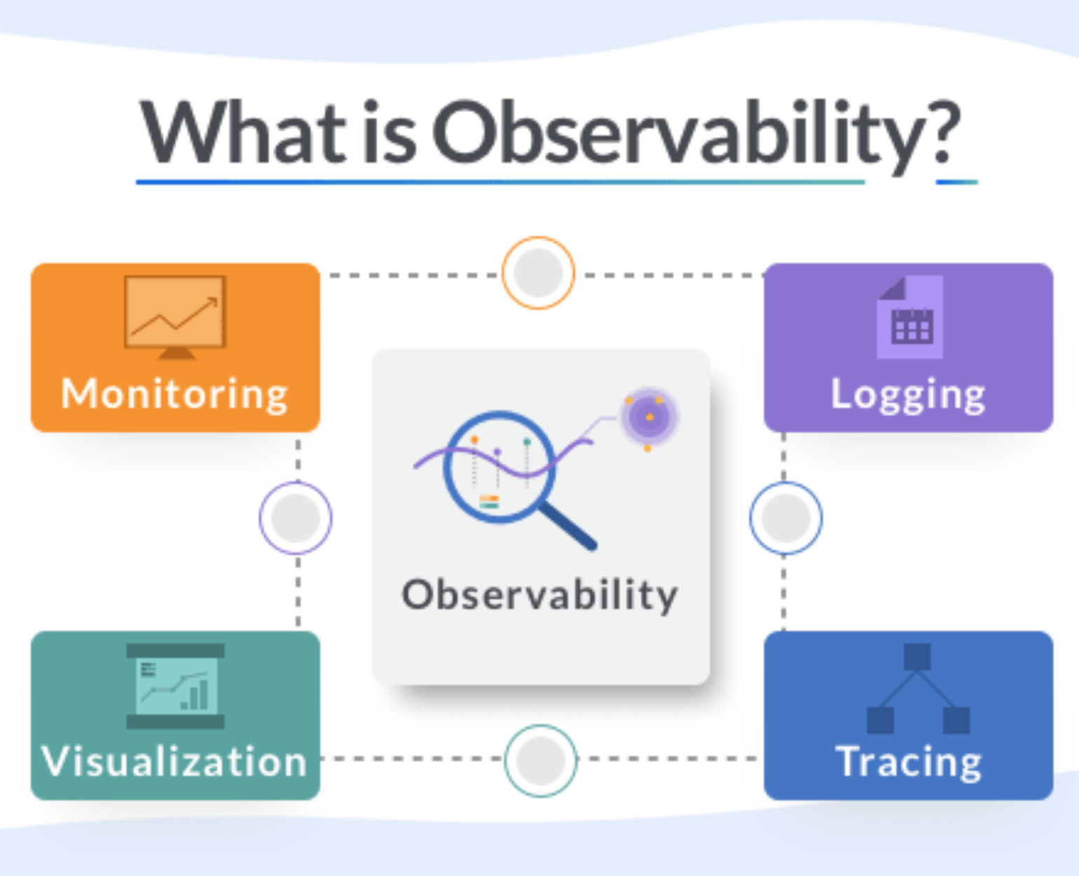
Core Definition and Evolution of Observability
Observability in software systems represents a paradigm shift from reactive to proactive operational management, enabling engineers to diagnose issues in complex, distributed environments by analyzing external data rather than relying on predefined metrics. Unlike traditional approaches, it emphasizes inferring system behavior through dynamic data collection, analysis, and contextual correlation. The evolution of observability reflects the growing complexity of modern architectures, where monolithic systems have given way to microservices, serverless functions, and edge computing—each introducing new layers of operational opacity.The foundational principles of observability were first articulated in control theory by Rudolf E. Kálmán in the 1960s, later adapted to software systems by engineers at companies like Google and Netflix. These principles distinguish observability from monitoring and logging by focusing on the reconstructability of system state from external outputs, rather than static metric thresholds or event logs. While monitoring tracks predefined KPIs (e.g., CPU usage, latency) and logging records discrete events, observability integrates these with distributed tracing, metrics, and logs to provide a holistic view of system behavior.
Foundational Principles of Observability
Observability in software systems is built on three core pillars: metrics, logs, and traces, collectively referred to as the "three pillars of observability." These pillars serve distinct but complementary roles in understanding system health and performance.- Metrics provide quantitative measurements (e.g., response time, error rates) at defined intervals, offering a high-level view of system behavior over time. Time-series data is critical for identifying trends, anomalies, and capacity planning.
The integration of these pillars enables contextual inference—the ability to derive the internal state of a system from external data. For example, a sudden spike in error logs (logs) paired with increased latency in a specific microservice (metrics) and a trace showing a dependency chain involving that service can pinpoint a root cause in a distributed environment.
Historical Progression and Key Milestones
The adoption of observability has evolved alongside the complexity of software architectures, with distinct phases marked by technological and methodological advancements.Pre-2010s: The Era of Monitoring and Logs
2010s: The Rise of Distributed Systems and Microservices
2020s: The Age of AI-Driven Observability and AIOps
Comparative Analysis: Observability vs. Monitoring vs. Logging
The distinction between observability, monitoring, and logging lies in their scope, data collection methods, and analytical capabilities. Below is a comparative table highlighting their primary focuses and key metrics collected:| Category | Primary Focus | Key Metrics Collected |
|---|---|---|
| Traditional Monitoring | Proactive detection of predefined issues using static thresholds and alerts. |
|
| Logging | Post-hoc debugging and auditing through structured or unstructured event records. |
|
| Observability | Inferring system state from dynamic, correlated data to enable proactive diagnostics. |
|
Influential Frameworks and Methodologies
Several frameworks and methodologies have shaped modern observability practices by introducing structured approaches to system reliability and operational excellence.Google’s Site Reliability Engineering (SRE)
Netflix’s Chaos Engineering
OpenTelemetry (OTel)
Core Tenet of Observability
Observability is the ability to infer the internal state of a system based on external outputs. Unlike monitoring, which relies on predefined metrics and alerts, observability enables engineers to diagnose issues in complex, distributed environments
Three Pillars of Observability: Metrics, Logs, and Traces
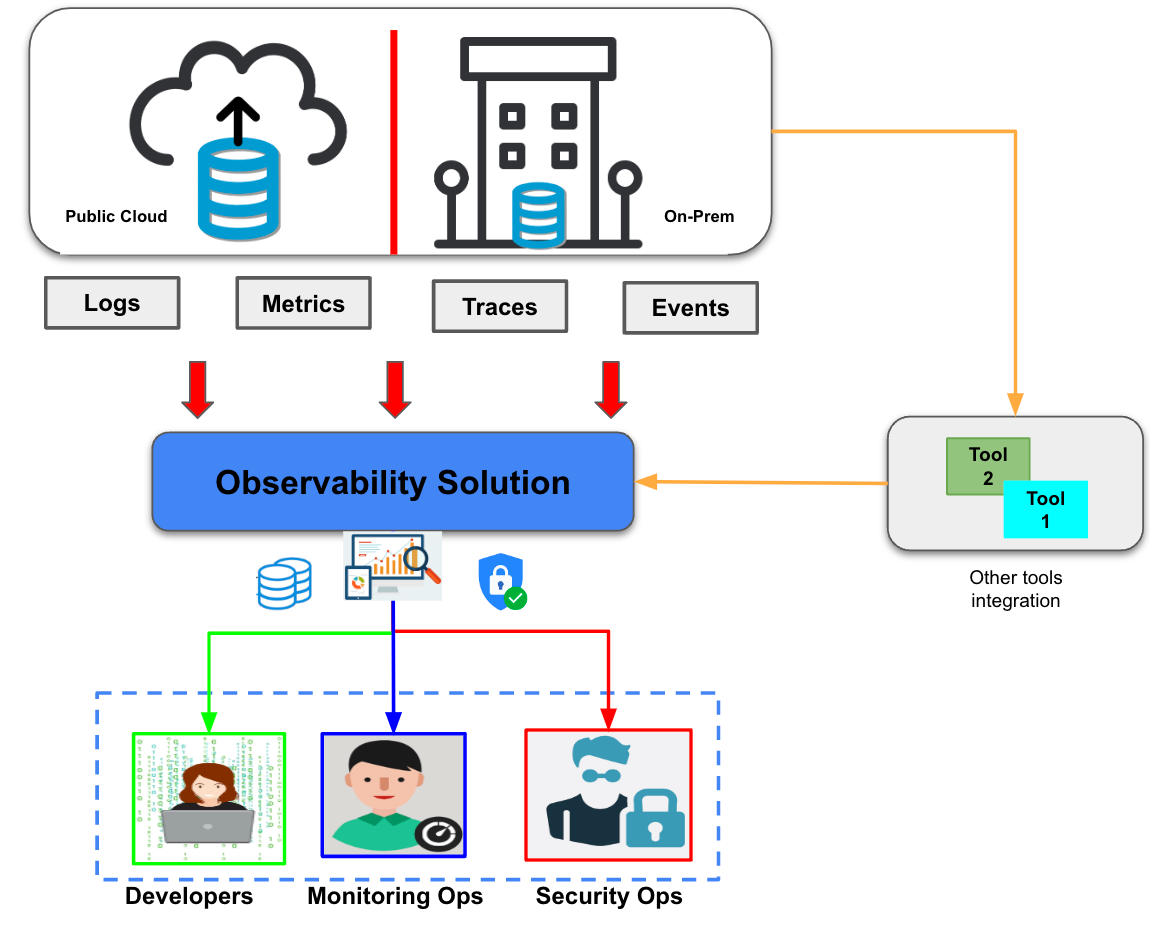
Observability in modern systems relies on three foundational pillars—metrics, logs, and traces—each serving distinct yet complementary roles in monitoring, debugging, and optimizing distributed architectures. Metrics provide quantitative snapshots of system health, logs offer granular, time-ordered narratives of events, and traces reconstruct end-to-end request flows across microservices. Together, they form a cohesive framework for understanding system behavior, identifying anomalies, and ensuring reliability at scale.The integration of these pillars enables organizations to transition from reactive troubleshooting to proactive observability, where real-time insights drive automated remediation and performance tuning. Below, each pillar is examined in depth, including its technical implementation, use cases, and integration with industry-standard tooling.
Metrics: Quantifying System Health with Time-Series Data
Metrics serve as the bedrock of observability by providing numerical measurements of system performance, resource utilization, and business outcomes. Unlike logs or traces, metrics are aggregated over time, enabling trend analysis, anomaly detection, and capacity planning. Critical metrics are categorized into four core dimensions:
Latency: Measures the time taken for operations (e.g., request processing, database queries). Traffic: Tracks the volume of requests, transactions, or data processed. Errors: Quantifies failures, exceptions, or retries (e.g., HTTP 5xx errors, timeouts). Saturation: Reflects resource constraints (e.g., CPU usage, memory leaks, queue depths). Example Time-Series Metrics:
Application Latency: `http_request_duration_seconds` (P99: 99th percentile latency). Error Rates: `error_rate` (e.g., `4xx_errors_total` or `database_connection_failed`). Resource Saturation: `system_cpu_usage_percent` or `container_memory_usage_bytes`. Business Metrics: `order_completion_rate` or `payment_failure_rate`. Metrics are typically collected via pull-based (e.g., Prometheus) or push-based (e.g., StatsD) mechanisms, with data stored in time-series databases (TSDBs) like InfluxDB or Thanos. Alerting rules (e.g., Prometheus Alertmanager) trigger notifications when thresholds (e.g., `latency > 500ms`) are breached, enabling preemptive action.
Metrics excel at answering what is happening (e.g., "The API latency spiked") but lack context on why it occurred.Logs: Structured and Unstructured Event Records for Debugging
Logs are sequential, timestamped records of events generated by applications, infrastructure, and services. They provide fine-grained visibility into system behavior, including user actions, configuration changes, and error conditions. Logs are classified into two primary formats:
Unstructured Logs: Human-readable text (e.g., `INFO: User logged in at 2023-10-01T12:00:00Z`). Structured Logs: Machine-parsable formats (e.g., JSON, `{"level":"INFO","timestamp":"2023-10-01T12:00:00Z","event":"user_login"}`). Use Cases for Logs:
Debugging: Tracing the lifecycle of a failed transaction by correlating logs across services. Forensics: Investigating security breaches or compliance violations (e.g., GDPR data access logs). Audit Trails: Tracking changes to critical configurations (e.g., Kubernetes manifest updates). User Behavior Analysis: Monitoring authentication flows or feature usage patterns. Log Management Workflow:
1. Collection: Agents (e.g., Fluentd, Filebeat) or SDKs (e.g., OpenTelemetry Logs) ingest logs from applications.
2. Processing: Parsing, enrichment (e.g., adding service metadata), and filtering (e.g., discarding debug logs in production).
3. Storage: Retention in centralized systems (e.g., ELK Stack, Loki, or Datadog).
4. Querying: Searching via tools like Kibana or Grafana Loki for patterns (e.g., `error AND service=payment`).
Structured logs enable automated parsing and correlation with metrics/traces, while unstructured logs preserve raw context for exploratory analysis.Distributed Traces: Mapping Request Flows Across Microservices
In microservices architectures, a single user request may traverse multiple services, databases, and third-party APIs. Distributed tracing captures the end-to-end journey of a request by instrumenting spans—timed, annotated segments representing individual operations (e.g., HTTP calls, database queries). Traces are structured hierarchically:
Root Span: Initiated by the client (e.g., a web request). Child Spans: Represent downstream calls (e.g., `auth_service`, `inventory_service`). Subspans: Granular operations within a service (e.g., `validate_token`, `fetch_product`). Key Components of a Trace:
Trace ID: Unique identifier for a request flow (e.g., `trace_id=abc123`). Span ID: Identifies individual operations (e.g., `span_id=xyz456`). Annotations: Metadata (e.g., `http.method=GET`, `db.query=SELECT FROM users`). Tags: Key-value pairs (e.g., `status_code=200`, `service=checkout`). Text-Based Trace Span Hierarchy Example:
Root Span (HTTP Request)
├── Span 1: auth_service.validate_token
│ ├── Subspan: jwt.decode
│ └── Subspan: user_db.lookup
├── Span 2: inventory_service.check_stock
│ └── Subspan: redis.get("product_123")
└── Span 3: payment_service.process
├── Subspan: stripe.charge
└── Subspan: order_db.createTools for Distributed Tracing:
OpenTelemetry: Vendor-neutral instrumentation library (supports auto-instrumentation for Java, Python, Go). Jaeger: Distributed tracing backend with UI for visualizing traces. Zipkin: Lightweight alternative with focus on low-overhead collection. Datadog APM: Commercial solution with advanced analytics. Traces reveal latency bottlenecks (e.g., a slow database query) and causal relationships between services (e.g., a timeout in `auth_service` cascading to `payment_service`).Comparison of Observability Pillars: Metrics, Logs, and Traces
The following table contrasts the three pillars across data type, use case, tooling ecosystem, and latency impact, highlighting their complementary roles in observability.
Pillar Data Type Use Case Tooling Ecosystem Latency Impact Metrics Time-series numerical data (e.g., counters, gauges, histograms) Monitoring system health, detecting anomalies, capacity planning Prometheus, Grafana, Thanos, Datadog Metrics, CloudWatch Low (aggregated, sampled) Structured key-value pairs (e.g., `service=checkout`, `status=success`) Alerting on SLOs (e.g., error budgets), trend analysis Alertmanager, VictoriaMetrics, InfluxDB Negligible (pull-based) Custom business metrics (e.g., `revenue_per_user`) Correlating business outcomes with technical performance Custom dashboards (Grafana), Mixpanel integration Moderate (requires transformation) Logs Unstructured text (e.g., `ERROR: Connection timeout`) Debugging, forensics, compliance auditing ELK Stack (Elasticsearch, Logstash, Kibana), Splunk, Loki High (storage-intensive, real-time indexing) Structured JSON/Protobuf (e.g., `{"event":"login
Observability in Distributed Systems and Microservices
Distributed systems and microservices architectures introduce complexity by decoupling components across networks, introducing non-deterministic behavior, and requiring real-time coordination. Traditional observability methods—such as centralized logging or simple metrics—fail to capture the dynamic interactions between services, leading to blind spots in failure detection, performance degradation, and dependency bottlenecks. Observability in these environments must address challenges like cascading failures, latency propagation, and service-to-service communication opacity, where a single misbehaving component can disrupt an entire system. Context propagation and distributed tracing emerge as critical enablers, while sampling strategies balance cost and coverage in high-throughput systems.The evolution of distributed architectures demands observability solutions that align with their inherent characteristics: statelessness, eventual consistency, and asynchronous communication. Without proper instrumentation, debugging becomes akin to solving a puzzle with missing pieces, where symptoms (e.g., HTTP 500 errors) obscure root causes (e.g., a database connection leak in a downstream service). Below, the focus shifts to addressing these challenges through technical mechanisms, trade-offs, and real-world implications.
Challenges in Distributed Architectures and Observability Requirements
Distributed systems amplify observability gaps due to their inherent complexity:
Cascading failures: A single service failure can trigger a domino effect across dependent services, obscuring the initial fault. Latency spikes: Network partitions or slow dependencies introduce unpredictable delays, making root-cause analysis difficult. Service dependencies: Tight coupling between services (e.g., synchronous calls) creates hidden bottlenecks that metrics alone cannot expose. Eventual consistency: Data inconsistencies across services complicate debugging, as state changes propagate asynchronously. Observability must provide temporal correlation (linking requests across services), causal tracing (mapping dependencies), and anomaly detection (identifying deviations in distributed workflows). Without these, teams rely on reactive debugging—post-mortems after outages—rather than proactive monitoring.
Challenge Observability Solution Example Scenario Cascading failures Distributed tracing with dependency mapping A payment service fails due to an unreachable inventory service, triggering rollbacks in order processing. Latency spikes End-to-end tracing with percentile analysis A 99th-percentile latency increase in a recommendation service degrades user experience. Service dependencies Context propagation for request correlation A user session ID must traverse authentication, cart, and checkout services to maintain consistency. Eventual consistency Event sourcing + trace correlation An order status update in a distributed ledger takes 10 seconds to propagate, causing UI staleness. Context Propagation and the W3C Trace Context Standard
Context propagation ensures that requests retain identity and metadata as they traverse services, enabling correlation across distributed components. Without it, logs and traces from individual services appear isolated, making it impossible to reconstruct end-to-end workflows. The W3C Trace Context standard (RFC 9163) defines a lightweight mechanism for propagating trace IDs, span IDs, and baggage (custom key-value pairs) via HTTP headers or message bags (e.g., Kafka headers, gRPC metadata).Key components of W3C Trace Context:
Trace ID: A globally unique identifier for a distributed transaction (e.g., a user request). Span ID: Identifies individual operations within a trace (e.g., a database query or API call). Baggage: User-defined key-value pairs (e.g., `tenant_id=acme`) attached to traces for correlation. Sampling flags: Control whether a trace is recorded (e.g., `sampled=1` for 100% sampling). The W3C Trace Context headers are:Implementation considerations:
`traceparent`: Contains the trace ID, parent span ID, sampled flag, and trace flags. `tracestate`: Extensible field for vendor-specific trace state (e.g., `datadog.env=prod`).
Header injection: Services must inject `traceparent` into outbound requests and extract it from inbound ones. Propagation formats: Support for multiple protocols (HTTP, gRPC, AMQP) via adapters or SDKs. Baggage limits: Custom baggage keys should be minimal to avoid performance overhead. Example workflow:
1. Client sends a request with a generated `traceparent` header.
2. Service A records a span, propagates the headers to Service B.
3. Service B appends its span to the trace, adds baggage (e.g., `user_role=admin`).
4. All logs and metrics for the trace include the `traceparent` for correlation.
Sampling Strategies for Traces in High-Throughput Systems
In systems processing millions of requests per second (e.g., e-commerce platforms, SaaS applications), recording every trace is infeasible due to storage costs and performance overhead. Sampling strategies balance coverage and resource usage, but incorrect choices lead to false negatives (missing critical failures) or false positives (over-instrumentation).Common sampling approaches:
100% sampling: Captures every request but scales poorly (e.g., 10,000 RPS → 10M traces/day). Probabilistic sampling: Randomly samples traces (e.g., 1% of requests) to reduce volume while preserving statistical significance. Adaptive sampling: Dynamically adjusts sampling rates based on system load or error rates (e.g., increase sampling during spikes). Head-based sampling: Samples based on request attributes (e.g., prioritize traces with `user_type=premium`). Trade-offs:
Best practices:
Strategy Pros Cons 100% sampling No missed critical traces; ideal for debugging. High storage costs; performance impact on agents. Probabilistic sampling Scalable; reduces storage costs by ~99%. May miss rare but critical failures (e.g., 0.1% error rate). Adaptive sampling Balances coverage and cost dynamically. Complex to implement; requires real-time metrics. Head-based sampling Targets high-value traces (e.g., VIP users). Requires business logic integration; may miss infrastructure issues.
Use probabilistic sampling as default (e.g., 1–5%) with adaptive overrides during incidents. Combine with error-based sampling: Always sample traces containing errors or latency outliers. Validate sampling effectiveness by comparing error rates in sampled vs. unsampled traces. Decision Flowchart for Selecting Observability Tools by System Complexity
Choosing observability tools depends on system architecture, scale, and operational requirements. Below is a text-based flowchart to guide selection:START
│
├─ Is the system a monolith?
│ ├─ Yes → Use centralized logging (e.g., ELK) + APM (e.g., New Relic)
│ │ ├─ Focus: Code-level metrics, slow query analysis
│ │ └─ End
│ └─ No → Proceed to distributed check
│
├─ Is the system microservices-based?
│ ├─ Yes → Use distributed tracing (e.g., Jaeger, OpenTelemetry)
│ │ ├─ Add context propagation (W3C Trace Context)
│ │ ├─ Implement sampling (probabilistic or adaptive)
│ │ └─ End
│ └─ No → Proceed to containerized check
│
├─ Is the system containerized (e.g., Kubernetes)?
│ ├─ Yes → Use service mesh (e.g., Istio, Linkerd) + eBPF (e.g., Pixie)
│ │ ├─ Integrate with metrics (Prometheus) and logs (Loki)
│ │ ├─ Enable distributed tracing for cross-pod workflows
│ │ └─ End
│ └─ No → Use traditional APM + custom instrumentation
│
└─ EndKey considerations:
Monoliths: Prioritize
Tools and Technologies for Implementing Observability
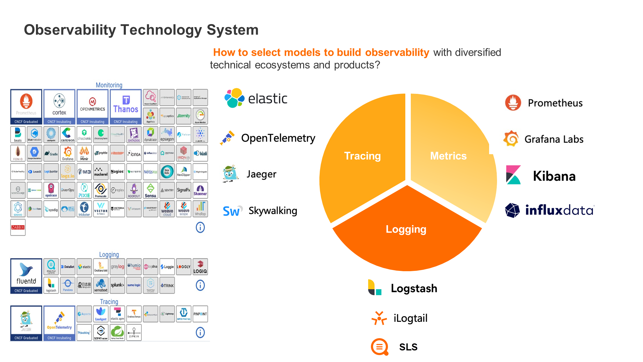
Observability in modern software systems relies on a combination of tools and technologies designed to collect, process, and analyze telemetry data. The choice between open-source and commercial solutions depends on factors such as cost efficiency, scalability requirements, and the need for advanced features like automated anomaly detection or integrated incident management. Below is a structured comparison of these platforms, along with essential components for building a robust observability stack and practical configurations for key tools.
Comparison of Open-Source and Commercial Observability Platforms
Open-source observability tools, such as Prometheus and Grafana, offer flexibility, cost-effectiveness, and community-driven innovation, making them ideal for organizations with technical expertise and customization needs. Commercial platforms like Datadog and New Relic, on the other hand, provide out-of-the-box integrations, managed services, and advanced analytics, reducing operational overhead but at a higher cost.Key Differences Across Platforms:
Example Scenarios:
Criteria Open-Source (Prometheus/Grafana) Commercial (Datadog/New Relic) Cost Free to use; self-hosted infrastructure costs apply. Subscription-based; pricing scales with usage (e.g., per host/metric). Scalability Requires manual scaling (e.g., Thanos for long-term storage). Auto-scaling with cloud-native support (e.g., Datadog’s distributed tracing). Feature Set Core metrics, logs, and traces; extensible via plugins. Full-stack observability, AIOps, synthetic monitoring, and SLO tracking. Ease of Deployment Self-managed; steep learning curve for configuration. Managed services with pre-configured dashboards and alerts. Integration Ecosystem Broad but requires custom scripting (e.g., Prometheus exporters). Native integrations with cloud providers, SaaS apps, and CI/CD tools. Use Case Fit Best for DevOps teams with control over infrastructure. Ideal for enterprises needing rapid deployment and vendor support.
Open-Source Suitability: Startups or mid-sized companies with Kubernetes clusters may prefer Prometheus + Grafana for cost savings and granular control over metrics retention. Commercial Suitability: Enterprises with multi-cloud deployments or compliance requirements often opt for Datadog or New Relic to avoid operational complexity and leverage AI-driven insights. Essential Components of a Modern Observability Stack
A comprehensive observability stack consists of interconnected layers responsible for collection, storage, querying, and alerting. Each component plays a critical role in ensuring real-time visibility into system health and performance.Collection Layer: Agents and Exporters
Data collection is the foundation of observability. Tools like Fluentd, Telegraf, and Prometheus Node Exporter ingest metrics, logs, and traces from applications and infrastructure. For example:
Fluentd excels in log aggregation with plugins for filtering and enrichment. Telegraf is lightweight and ideal for collecting metrics from databases, cloud providers, and IoT devices. Prometheus exporters (e.g., `node_exporter`, `blackbox_exporter`) expose system-level metrics in a standardized format. Storage Layer: Time-Series and Log Databases
Efficient storage ensures query performance and cost optimization. Solutions include:
Thanos for Prometheus long-term storage and high availability. ClickHouse for high-performance analytics on logs and metrics. Elasticsearch for full-text search and log correlation (commonly paired with the ELK Stack). Querying Layer: Languages and Interfaces
Querying tools enable exploration and visualization of telemetry data. Key examples:
PromQL (Prometheus Query Language) for metric-based queries with functions like `rate()`, `sum()`, and `group_by()`. Grafana as a unified interface for dashboards, supporting multiple data sources (Prometheus, Elasticsearch, etc.). Loki Query Language (LogQL) for log-based queries in Grafana. Alerting Layer: Rules and Integrations
Alerting transforms raw data into actionable insights. Components include:
Alertmanager (Prometheus) for deduplication and routing alerts to platforms like PagerDuty or Slack. Custom alerting rules in PromQL (e.g., `alert if error_rate > 0.1`). Synthetic monitoring tools (e.g., Datadog Synthetics) to simulate user interactions and detect availability issues. Configuring Prometheus for a Node.js Application
Prometheus scrapes metrics from exposed endpoints (typically `/metrics`) using a scrape configuration file (`prometheus.yml`). Below is an example configuration for a Node.js app running on port `3000`, with relabeling and metric exclusion rules.global:
scrape_interval: 15s
evaluation_interval: 15sscrape_configs:
job_name: 'nodejs_app' static_configs:
targets: ['localhost:3000'] metrics_path: '/metrics'
relabel_configs:
source_labels: [__address__] target_label: 'instance'
regex: '(.+)'
replacement: '${1}'
source_labels: [job] regex: 'nodejs_app'
target_label: 'app'
replacement: 'user-service'
metric_relabel_configs:
action: drop regex: 'nodejs_go_gc_duration_seconds'
source_labels: [__name__]Key Configurations Explained:
`job_name`: Identifies the target application in Prometheus. `relabel_configs`: Renames or modifies labels (e.g., `instance` for host identification). `metric_relabel_configs`: Excludes irrelevant metrics (e.g., Go garbage collection metrics if using a non-Go Node.js app). `metrics_path`: Specifies the endpoint where the Node.js app exposes metrics (e.g., via `prom-client` library). Prerequisites for Node.js:
1. Install the `prom-client` library:npm install prom-client
2. Expose metrics in your app:
const client = require('prom-client');
const collectDefaultMetrics = client.collectDefaultMetrics;
collectDefaultMetrics({ timeout: 5000 });
app.get('/metrics', async (req, res) => {
res.set('Content-Type', client.register.contentType);
res.end(await client.register.metrics());
});
Grafana Dashboard Template for SLOs and Error Budgets
Service Level Objectives (SLOs) and error budgets quantify reliability and guide incident prioritization. Below is a Grafana dashboard template visualizing:
SLO Compliance: Percentage of successful requests over a time window. Error Budget: Remaining budget before declaring a service degradation. Latency Percentiles: P95/P99 response times. Dashboard Panels:
1. SLO Compliance (Time Series)
Query: `sum(rate(http_requests_total{status=~"2.."}[5m])) / sum(rate(http_requests_total[5m]))` Threshold: Compare against the SLO target (e.g., 99.9% availability). Visualization: Line graph with a static line for the SLO target. 2. Error Budget (Gauge)
Query: `(1 - SLO_compliance) 100` Threshold: Highlight when the budget is exhausted (e.g., > 0.1% errors). Visualization: Gauge with red/yellow/green zones. 3. Latency Distribution (Histogram)
Query: `histogram_quantile(0.95, sum(rate(http_request_duration_seconds_bucket[5m])) by (le))` Visualization: Bar chart with buckets for P95, P99, and P99.9. Example PromQL for Error Budget Calculation:
(
sum(rate(http_requests_total{status=~"5.."}[5m]))
/
sum(rate(http_requests_total[5m]))
) 100 > 0.1Note: Replace `http_requests_total` with metrics relevant to your Node.js app (e.g., `nodejs_http_requests_total`).
Role of AIOps in Augmenting Observability
Artificial Intelligence for IT Operations (AIOps) enhances observability by automating anomaly detection, correlating events across silos, and providing predictive insights. Tools like Dynatrace and Splunk leverage machine learning to reduce alert noise and accelerate root cause analysis (RCA).Key AIOps Capabilities:
Observability is not merely a toolset but a cultural and technical imperative for organizations navigating the scale and velocity of modern infrastructure. From the foundational distinction between monitoring and inferential analysis to the strategic integration of traces in distributed systems, its adoption demands a holistic approach—spanning instrumentation, tooling, and operational practices. The shift toward probabilistic sampling, AIOps-driven anomaly detection, and standardized frameworks like OpenTelemetry underscores a broader trend: systems must be designed with observability in mind, not bolted on as an afterthought. As teams grapple with increasingly complex architectures, the ability to see beyond surface-level metrics will define the difference between reactive firefighting and proactive mastery of system behavior.
FAQ
what is observability in software?
Q: What exactly is observability in software, and how does it differ from traditional monitoring?
what is observability in ai?
Q: How does observability apply specifically to AI systems, and why is it important?
what is observability in devops?
Q: What role does observability play in DevOps practices, and how is it implemented?
what is observability in agentic ai?
Q: What is observability in the context of agentic AI, and what challenges does it pose?
what is observability and monitoring?
Q: What’s the difference between observability and monitoring, and when should you use each?
what is observability in tech?
Q: How is observability defined in the broader tech industry, beyond software engineering?
Leave a Comment
Comments are moderated before appearing. The data you submit is processed according to the Privacy Policy of Voltefac.