Stars Are Made Of What Core Elements And Processes Behind Them
Table of Contents
- Composition of Stars: The Core Elements and Stellar Nucleosynthesis
- Elemental Composition of Stars by Stellar Phase
- Stages of Stellar Nucleosynthesis
- Physical States and Conditions Inside Stars
- Extreme Temperatures and Pressures in Stellar Cores
- Plasma States in Stars vs. Other Celestial Bodies
- Convection and Radiation Zones: Energy Transport Mechanisms
- Magnetic Fields in Stellar Atmospheres and Stellar Activity
- Observational Evidence: Spectroscopy and Stellar Classification
- Spectroscopy: Decoding Stellar Composition Through Light
- Comparison of Stellar Spectra: Elements and Characteristics by Spectral Type
- Theoretical Models: Simulating Stellar Formation and Evolution
- Stellar Formation Models: From Molecular Clouds to Protostars
- Computational Simulations of Elemental Distribution During Stellar Lifecycles
- Structured Outline of a Hypothetical Star’s Evolution with Compositional Changes
- Comparing Theoretical Models with Observational Data
- Visualizing Stellar Composition: Diagrams and Data Representations
- Interpreting Spectral Lines to Deduce Elemental Abundance
- Interactive Elemental Abundance Table Across Star Types
- Generating a 3D Model of a Star’s Interior with Compositional Layers
- Practical Applications of Stellar Composition in Astronomy and Technology
- Stellar Composition and Planetary System Formation
- Spectroscopy and the Detection of Exoplanets with Habitable Potential
- Technologies for Analyzing Stellar Elements
- Historical Foundations and Modern Legacy
- FAQ
- What elements are stars made of?
- What gas are stars made of?
- What gases are stars made of?
- What are stars composed of?
- What are stars mostly made of?
- What are shooting stars made of?
The composition of stars is a fundamental pillar of astrophysics, revealing the cosmic alchemy that transforms simple elements into the building blocks of galaxies, planets, and life itself. At their cores, stars are vast nuclear furnaces where hydrogen and helium undergo fusion under extreme pressures, synthesizing heavier elements that enrich the universe. From the birth of a protostar in a molecular cloud to the explosive death of a supernova, each stage reshapes stellar chemistry, leaving behind remnants that hold clues to cosmic evolution. This exploration examines the elemental origins of stars, the physical forces governing their interiors, and how spectroscopic observations decode their secrets—bridging theoretical models with cutting-edge astronomical discoveries.
Understanding what stars are made of extends beyond academic curiosity; it illuminates the origins of planetary systems, the potential for habitable worlds, and the technological advancements that enable modern astrophysics. Through simulations, spectral analysis, and historical observations, scientists trace the lifecycle of elements from stellar nucleosynthesis to their dispersion across space, shaping the very matter that surrounds us. This discussion synthesizes empirical data, theoretical frameworks, and observational techniques to unravel the intricate tapestry of stellar composition and its profound implications for the cosmos.
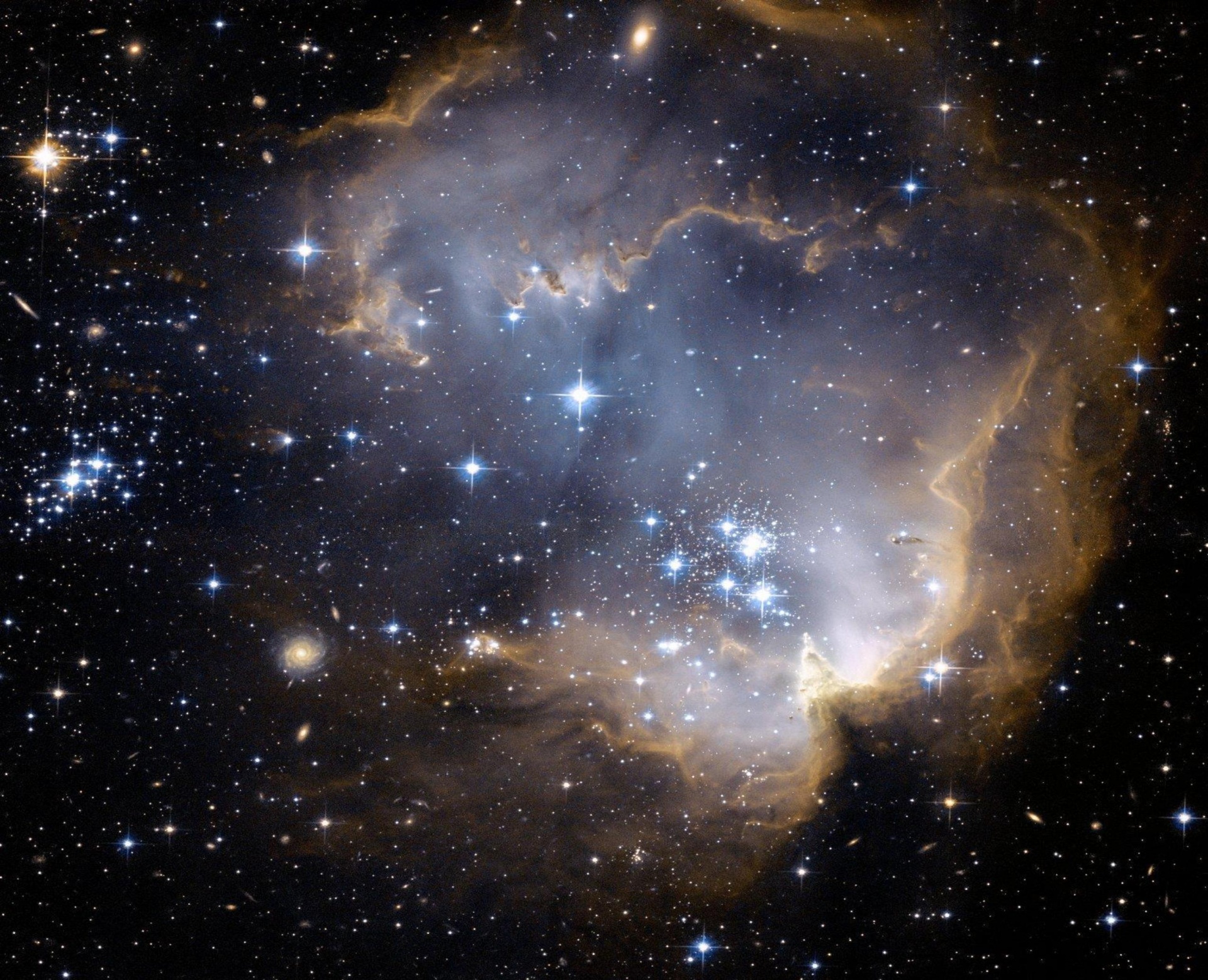
Composition of Stars: The Core Elements and Stellar Nucleosynthesis
Stars are primarily composed of hydrogen (approximately 70–75% by mass) and helium (23–28% by mass), with trace amounts of heavier elements (~0.1–2% by mass), collectively termed metallicity in astrophysics. These heavier elements—such as carbon, oxygen, neon, magnesium, silicon, iron, and trace quantities of gold, uranium, and others—originate from stellar nucleosynthesis, the process by which lighter elements fuse into heavier ones under extreme temperatures and pressures. The elemental composition of a star evolves over its lifecycle, transitioning from hydrogen-dominated main-sequence phases to helium-rich red giant stages, and ultimately dispersing enriched material through stellar winds or explosive supernovae. This distribution seeds the interstellar medium with the building blocks for new stars, planets, and life.The synthesis of elements in stars follows a hierarchical progression, governed by nuclear fusion reactions that release energy while transforming atomic nuclei. Hydrogen fusion dominates in main-sequence stars, while advanced stages involve helium burning, carbon fusion, and the formation of elements up to iron via the triple-alpha process, CNO cycle, and silicon burning. Beyond iron, neutron capture processes (s-process and r-process) produce the heaviest elements during supernovae or neutron star mergers. Below, the stages of nucleosynthesis are detailed, followed by a comparative analysis of elemental distributions across stellar lifecycles and the mechanisms by which these elements are dispersed into space.
Elemental Composition of Stars by Stellar Phase
The relative abundance of elements in stars varies significantly depending on their evolutionary stage, mass, and metallicity. Below is a comparative table summarizing the approximate elemental composition (by mass) of three distinct stellar phases: main-sequence stars, red giants, and supernova remnants. Data is derived from spectroscopic observations and stellar evolution models, with variations accounting for stellar mass and initial metallicity.| Element | Main-Sequence Stars (e.g., Sun-like, ~1 M☉) | Red Giants (Post-main-sequence, ~1–8 M☉) | Supernova Remnants (Type II, ~8–50 M☉) |
|---|---|---|---|
| Hydrogen (H) | ~73% | ~20–50% (core depletion) | ~0–10% (dispersed) |
| Helium (He) | ~25% | ~50–70% (helium core) | ~10–30% (enriched) |
| Carbon (C) | ~0.3% | ~1–5% (triple-alpha products) | ~1–3% (synthesized) |
| Oxygen (O) | ~0.7% | ~1–3% | ~2–5% |
| Neon (Ne) | ~0.1% | ~0.5–1% | ~1–2% |
| Magnesium (Mg) | ~0.05% | ~0.1–0.5% | ~0.5–1% |
| Silicon (Si) | ~0.03% | ~0.05–0.2% | ~1–3% (silicon burning) |
| Iron (Fe) | ~0.15% | ~0.2–0.5% | ~5–10% (peak abundance) |
| Nickel (Ni) | ~0.02% | ~0.03% | ~1–2% (decays to Fe) |
| Heavier Elements (Z > 26) | ~0.01% | ~0.02–0.1% | ~0.1–1% (r-process/s-process) |
Stages of Stellar Nucleosynthesis
The synthesis of elements in stars proceeds through distinct phases, each triggered by rising core temperatures and pressures. The progression can be summarized as follows:-
Proton-Proton Chain (PPC) and CNO Cycle (Main-Sequence Phase)
Stars spend ~90% of their lifecycles fusing hydrogen into helium via the PPC (dominant in low-mass stars) or the CNO cycle (predominant in high-mass stars). The PPC converts four protons into helium-4, releasing energy and neutrinos:41H → 4He + 2e+ + 2νe + 2γ + 26.7 MeV.
The CNO cycle catalyzes fusion using carbon-12 as an intermediary, accelerating energy production in massive stars. -
Helium Burning (Triple-Alpha Process, Red Giant Phase)
Once core hydrogen is depleted, gravitational collapse raises temperatures to ~100 million K, enabling helium fusion. The triple-alpha process combines three helium-4 nuclei into carbon-12:34He → 12C + γ + 7.27 MeV.
Further reactions produce oxygen-16, neon-20, and magnesium-24. This phase also generates trace amounts of beryllium-7 and lithium-7 via side reactions. -
Advanced Burning: Carbon, Neon, Oxygen, and Silicon Fusion
In stars with masses >8 M☉, carbon ignition (at ~600 million K) initiates the synthesis of heavier elements:- Carbon Burning (600–1,000 million K): Fuses carbon into neon, sodium, and magnesium.
- Neon Burning (1,000–1,500 million K): Photodisintegrates neon into oxygen and magnesium, releasing energy.
- Oxygen Burning (1,500–3,000 million K): Produces silicon, sulfur, and phosphorus.
- Silicon Burning (3,000–5,000 million K): Rapidly synthesizes iron-peak elements (chromium to nickel) via photodisintegration and alpha capture.
-
Neutron Capture Processes (Supernovae and Neutron Star Mergers)
Elements beyond iron are produced via neutron capture:- Slow Neutron-Capture Process (s-process): Occurs in asymptotic giant branch
Physical States and Conditions Inside Stars
The interiors of stars represent environments of extreme physical conditions, where matter exists in states fundamentally distinct from those encountered on Earth or in most other celestial bodies. These conditions—ranging from temperatures exceeding millions of Kelvin to pressures millions of times greater than Earth’s atmospheric pressure—enable processes such as nuclear fusion, energy transport, and the generation of magnetic fields. Understanding these states is critical to comprehending stellar evolution, energy production, and the dynamic behavior observed in stellar atmospheres. The following sections explore the core conditions, plasma states, energy transport mechanisms, and the role of magnetic fields in shaping stellar phenomena.
Extreme Temperatures and Pressures in Stellar Cores
The cores of main-sequence stars, particularly those of spectral types O, B, A, and F, sustain temperatures exceeding 10 million Kelvin (K), with massive stars (e.g., O-type) reaching 40 million K or higher. These temperatures are a direct consequence of gravitational compression, where the inward pull of a star’s mass generates pressures sufficient to overcome Coulomb barriers in atomic nuclei. At such extremes, hydrogen nuclei (protons) undergo proton-proton chain reactions or, in higher-mass stars, the CNO cycle, converting hydrogen into helium while releasing energy via Einstein’s mass-energy equivalence (E = mc²).Pressure in stellar cores follows a hydrostatic equilibrium, balancing gravitational collapse with outward radiation pressure. For a star like the Sun, core pressures reach ~250 billion atmospheres (2.5 × 10¹⁶ Pa), while in massive stars, these values can exceed 10¹⁸ Pa. These conditions ensure that fusion reactions proceed at rates sufficient to counteract gravitational contraction, maintaining stellar stability over billions of years. The relationship between temperature (T), pressure (P), and density (ρ) is governed by the ideal gas law (PV = nRT) and radiative transfer equations, modified for degenerate matter in late-stage stars.
Key Fusion Thresholds:
- Proton-proton chain (P-P chain): Dominant in stars ≤1.3 M☉; requires ~10–15 million K.
- CNO cycle: Predominant in stars >1.3 M☉; efficient at ~15–20 million K.
- Helium burning (triple-alpha process): Initiates at ~100 million K, producing carbon and oxygen.
- Granulation: Small-scale convection cells (~1,000 km) in the Sun’s photosphere, with 5-minute oscillation periods.
- Supergranulation: Larger cells (~30,000 km) linked to horizontal flows in the upper convection zone.
- Meridional Circulation: Poleward flow of plasma, influencing differential rotation and magnetic field topology.
- Low-mass stars (M < 1.1 *M☉): Fully convective interiors (e.g., red dwarfs).
- High-mass stars (M > 1.3 *M☉): Thin convection zones near the surface, with radiative cores dominated by the CNO cycle.
- α-effect: Twisting of field lines by helical turbulence in the convection zone (e.g., cyclonic motions).
- Ω-effect: Stretching of fields by differential rotation (faster equator than poles). Combined, these processes generate large-scale toroidal and poloidal fields, as modeled in the Babcock-Leighton paradigm for solar activity.
- Operates in granular convection, producing kG-strength fields in starspots.
- Dominant in fully convective stars (e.g., M dwarfs), where large-scale fields are weaker but frequent flaring occurs.
- Starspots: Dark, cool (~1,500 K below photospheric temperature) regions caused by magnetic suppression of convection. Their distribution follows active latitudes (e.g., Sun’s Butterfly Diagram), migrating toward the equator over activity cycles (e.g., 11-year solar cycle).
- Continuum Spectrum: The broad, uninterrupted range of wavelengths emitted by a star’s photosphere, modified by temperature and opacity.
- Absorption Lines: Dark bands at discrete wavelengths where photons are absorbed by atoms or molecules in the stellar atmosphere.
- Emission Lines: Bright lines superimposed on the continuum, typically observed in active regions or surrounding gas clouds.
- Molecular Bands: Broadened absorption features caused by complex molecules (e.g., TiO in M-type stars), indicating cooler temperatures where molecules can form.
- Strong He II λ4686 emission (Wolf-Rayet stars).
- Weak or absent Balmer lines (Hα, Hβ).
- UV resonance lines of C, N, O.
- Prominent Balmer series (Hα, Hβ).
- He I lines (e.g., λ4471, λ5876).
- Weaker metal lines compared to A-type.
- Strongest Balmer lines (Hα dominant).
- Ca II H/K lines.
- Metallic lines (Fe, Mg) begin to appear.
- Weakening Balmer series.
- Strong Ca II H/K and G-band (CH).
- Iron-peak elements (Fe, Cr) prominent.
- Weak Hα, strong Ca II.
- Iron and molecular bands (e.g., CN in K-type giants).
- Solar-type stars show Fraunhofer lines.
- Strong TiO bands (red/orange stars).
- Weak Hα, prominent metal lines.
- Molecular features (e.g., VO in late K).
-
Theoretical Models: Simulating Stellar Formation and Evolution
Stellar formation and evolution are governed by complex physical processes, from gravitational collapse in molecular clouds to nuclear fusion in stellar cores. Theoretical models integrate hydrodynamics, radiative transfer, and nuclear physics to simulate these stages, while computational simulations predict elemental distributions across a star’s lifecycle. Key processes, such as the CNO cycle and the triple-alpha reaction, are validated against observational data, though discrepancies often arise due to uncertainties in initial conditions or unresolved physical phenomena. Below, the structured progression of stellar formation, elemental accumulation, and lifecycle simulations are examined, alongside comparisons between theoretical predictions and empirical evidence.
Stellar Formation Models: From Molecular Clouds to Protostars
The formation of a star begins in dense molecular clouds, where gravitational instability triggers collapse under self-gravity. Theoretical models decompose this process into stages, emphasizing the accumulation of elements from the interstellar medium (ISM) into the collapsing core. Key steps include:
Jeans Instability Criterion (λ_J):
The critical wavelength beyond which a cloud fragment collapses under gravity:
\[
\lambda_J = \sqrt{\frac{\pi c_s^2}{G \rho}},
\]
where \(c_s\) is the sound speed, \(G\) is the gravitational constant, and \(\rho\) is the cloud density.-
Initial Cloud Fragmentation:
Molecular clouds (e.g., in Orion or Taurus-Auriga) exhibit turbulent density fluctuations. Numerical simulations (e.g., using smoothed particle hydrodynamics, SPH) resolve fragmentation into cores with masses ~0.1–10 \(M_{\odot}\). Elemental abundances in these cores reflect the ISM composition, enriched by prior stellar nucleosynthesis (e.g., supernova ejecta). -
Isothermal Collapse and Protostar Formation:
As a core collapses, gravitational energy converts to thermal energy, raising temperatures to ~10–20 K. Accretion disks form, funneling material onto the central protostar. Spectroscopic observations (e.g., ALMA data of Class 0/I protostars) confirm infall velocities and dust enrichment, where heavier elements (e.g., Si, Fe) condense into grains, altering opacity and cooling rates. -
Kelvin-Helmholtz Contraction and Deuterium Burning:
Protostars reach ~1,000 K, initiating deuterium fusion (D + p → \(^3\)He + γ), a transient phase lasting ~10^4–10^5 years. This stage accumulates hydrogen and helium while depleting deuterium, setting the stage for hydrogen burning. Simulations (e.g., MESA stellar evolution code) track this transition, showing how protostellar winds and outflows regulate accretion rates and elemental mixing.
Computational Simulations of Elemental Distribution During Stellar Lifecycles
Stellar nucleosynthesis models predict how elements are synthesized and distributed across a star’s lifecycle, with computational simulations (e.g., 1D stellar evolution codes like MESA or 3D hydrodynamic models like PROMETHEUS) resolving these processes. Key nuclear pathways and their simulation outputs include:
Triple-Alpha Process (Helium Burning):
Three helium-4 nuclei fuse to form carbon-12 via an unstable beryllium-8 intermediate:
\[
3 \, ^4\text{He} \rightarrow ^{12}\text{C} + \gamma + 7.275 \, \text{MeV}.
\]
This process dominates in stars >0.5 \(M_{\odot}\) and enriches the core with carbon and oxygen, later fueling the CNO cycle.-
Hydrogen Burning Phase (Main Sequence):
Stars spend ~90% of their lifetimes fusing hydrogen via the proton-proton chain (dominant in stars <1.3 \(M_{\odot}\)) or the CNO cycle (dominant in higher-mass stars). Simulations show how the CNO cycle catalyzes hydrogen burning, increasing the abundance of \(^{14}\)N, \(^{16}\)O, and \(^{17}\)O while depleting \(^{12}\)C. Observational confirmation comes from spectroscopic abundances in solar-type stars (e.g., the Sun’s photospheric nitrogen excess). -
Helium Core Burning and Beyond:
As hydrogen is exhausted, the core contracts and heats to ~10^8 K, igniting helium via the triple-alpha process. Simulations predict the formation of a degenerate carbon-oxygen core in stars <8 \(M_{\odot}\), while higher-mass stars undergo additional burning stages (e.g., neon, oxygen, silicon) leading to iron-peak elements. The distribution of these elements is tracked via nucleosynthesis yields, which are compared to meteoritic and stellar abundance data (e.g., the solar system’s silicon-to-iron ratio). -
Late-Stage Mixing and Mass Loss:
In asymptotic giant branch (AGB) stars, convection dredges up carbon and s-process elements (e.g., \(^{13}\)C, \(^{22}\)Ne) to the surface, enriching the circumstellar envelope. Simulations (e.g., MONASH code) model this mixing, predicting isotopic ratios (e.g., \(^{12}\)C/\(^{13}\)C) that match observations in planetary nebulae (e.g., the Ring Nebula’s carbon-rich ejecta).
Structured Outline of a Hypothetical Star’s Evolution with Compositional Changes
The lifecycle of a 5 \(M_{\odot}\) star illustrates key compositional transitions, from molecular cloud collapse to supernova enrichment. Below is a structured outline with simulation-derived predictions:
Stage Dominant Processes Elemental Changes Observational/Simulation Evidence Molecular Cloud Collapse Gravitational fragmentation, accretion ISM composition (H:He ~75:25 by mass, trace metals from prior supernovae) ALMA observations of dust continuum emission in star-forming regions (e.g., Perseus Molecular Cloud). Protostar Phase (Class 0/I) Deuterium burning, K-H contraction Deuterium depletion; H/He ratio preserved; dust grains form (Si, Fe, Mg). Infrared excess in Spitzer/IRAS data; MESA simulations of pre-main-sequence evolution. Main Sequence (Hydrogen Burning) CNO cycle (dominant) \(^{12}\)C → \(^{14}\)N → \(^{16}\)O; \(^{16}\)O/\(^{17}\)O ratio increases. Spectroscopic abundances in B-type stars (e.g., \(^{14}\)N/\(^{16}\)O > 1 in fast-rotating stars). Red Giant Branch (Helium Ignition) Triple-alpha process, shell hydrogen burning Core: \(^{12}\)C, \(^{16}\)O; envelope enriched in \(^{13}\)C (s-process). Carbon stars (e.g., IRC +10216) with \(^{12}\)C/\(^{13}\)C ~10–50. Supernova Explosion Silicon burning, explosive nucleosynthesis Iron-peak elements (Fe, Ni); neutron-capture elements (Sr, Ba) via r-process. Supernova remnants (e.g., Cassiopeia A) with X-ray emission lines of Si, S, Ar. Comparing Theoretical Models with Observational Data
Theoretical stellar models rely on assumptions about mixing, rotation, and nuclear reaction rates, which are tested against empirical data. Key comparisons include:
-
Solar Abundance Problem:
Standard solar models predict a higher \(^{12}\)C/\(^{16}\)O ratio than observed (~0.5 vs. ~0.4). This discrepancy suggests unresolved mixing processes or uncertainties in the \(^{12}\)C(α,γ)\(^{16}\)O reaction rate. Simulations incorporating rotation or magnetic fields (e.g., ESTER

Visualizing Stellar Composition: Diagrams and Data Representations
Stellar composition is not directly observable but can be inferred through spectroscopic analysis, theoretical models, and computational simulations. These methods reveal the elemental abundances, physical conditions, and evolutionary stages of stars, from their cores to their outer layers. Visual representations—such as spectral line diagrams, interactive abundance tables, and 3D interior models—bridge observational data with theoretical frameworks, enabling astronomers to reconstruct the chemical and structural profiles of stars and their remnants.The interpretation of stellar spectra serves as the foundation for deducing elemental composition. Spectral lines, formed by electron transitions in atoms and ions, act as fingerprints that identify elements and their ionization states. High-resolution spectrographs decompose starlight into discrete wavelengths, where absorption or emission lines correspond to specific elements. For instance, the Balmer series in hydrogen (Hα, Hβ) dominates in cooler stars, while iron (Fe II, Fe III) and calcium (Ca II) lines become prominent in hotter or more evolved stars. The strength and width of these lines, influenced by temperature, pressure, and turbulence, further refine abundance estimates.
Interpreting Spectral Lines to Deduce Elemental Abundance
Spectroscopy reveals the chemical composition of stars by analyzing the absorption or emission lines in their spectra. Each element absorbs or emits light at characteristic wavelengths, producing a unique spectral signature. The Kirchhoff’s laws of spectral analysis provide the theoretical basis:
- Absorption lines occur when photons are absorbed by atoms in the star’s outer layers, exciting electrons to higher energy levels.
- Emission lines arise in nebulae or stellar atmospheres where electrons transition back to lower states, releasing energy as light.
Key spectral features for elemental identification include:
- Hydrogen lines (Balmer series, Lyman series): Dominant in main-sequence stars, particularly A-type stars (e.g., Sirius).
- Helium lines (He I, He II): Visible in O- and B-type stars, indicating high temperatures and nuclear fusion processes.
- Metal lines (Fe, Ca, Mg, Si): Abundant in cooler stars (F, G, K types) and stellar remnants, reflecting nucleosynthesis products.
- Molecular bands (CN, CH, TiO): Present in M-type stars, indicating low temperatures where molecules form in the photosphere.
The equivalent width of a spectral line—measured as the width of a rectangular absorption profile with the same area—quantifies the abundance of an element. Combined with curve-of-growth analysis, astronomers derive logarithmic abundances (e.g., [Fe/H], where [X/Y] = log₁₀(Nₓ/Nₜ) – log₁₀(Nₓ/Nₜ)⊙). For example, a star with [Fe/H] = +0.3 has 2 times the solar iron abundance, while [Fe/H] = –1.0 indicates 10% of the solar value.
Interactive Elemental Abundance Table Across Star Types
The following table presents the relative abundances of key elements in different spectral types, normalized to hydrogen (H = 10⁶). Data are derived from stellar atmosphere models and high-resolution spectroscopy (e.g., Asplund et al. (2009), Caffau et al. (2011)). The table includes main-sequence stars, red giants, and stellar remnants, illustrating how nucleosynthesis and mixing processes alter composition over a star’s lifetime.
Notes:Element O-type (Hot, Massive) G-type (Sun-like) M-type (Cool, Low-Mass) White Dwarf (Post-AGB) Neutron Star (Core Remnant) Hydrogen (H) 700,000 920,000 760,000 0 (depleted) Trace (crust) Helium (He) 280,000 70,000 230,000 99.9% (He core) Trace (superfluid) Carbon (C) 1,000 4,600 1,500 0.1% (surface layers) 0.01% (crust) Oxygen (O) 2,000 8,500 3,000 0.01% (mixed) Trace (nuclear pasta) Iron (Fe) 100 4,600 150 0.001% (metal-rich core) 50% (crust composition) Neon (Ne) 5,000 1,200 500 Trace (degenerate core) 10% (inner crust) Silicon (Si) 1,000 5,000 100 0.0001% 20% (crust)
- Abundances are logarithmic (scaled to H = 10⁶ for clarity).
- White dwarfs show hydrogen depletion due to shell burning; helium dominates in their cores.
- Neutron stars exhibit extreme enrichment of heavy elements (e.g., iron, silicon) in their crusts, formed via neutron capture and nuclear reactions during supernovae.
Generating a 3D Model of a Star’s Interior with Compositional Layers
A 3D stellar interior model visualizes temperature gradients, density stratification, and elemental distribution across radial layers. Such models integrate observational constraints (e.g., helioseismology for the Sun, asteroseismology for other stars) with theoretical equations of state and nuclear reaction networks. Below are steps to construct and interpret a simplified model using computational tools like MESA (Modules for Experiments in Stellar Astrophysics) or STARLIB.Key Layers and Their Compositional Features:
1. Core:
- Temperature: 10–15 million K (main-sequence), up to 100 million K (advanced stages).
- Composition: Primarily hydrogen (early stages) or helium/ash from fusion (e.g., C, O, Ne, Fe in later stages).
- Processes: Proton-proton chain (low-mass stars) or CNO cycle (high-mass stars); neutron capture in AGB stars.
- Visualization: High-density, radiative core with sharp compositional gradients at fusion boundaries.
2. Radiative Zone:
- Temperature: 2–7 million K, decreasing outward.
- Composition: Gradual mixing of fusion products (e.g., helium ash in the Sun).
- Processes: Energy transport via photon diffusion; minimal convection.
- Visualization: Smooth temperature decline with layered abundance profiles (e.g., [He/H] increasing inward).
3. Convective Zone:
- Temperature: <2 million K (outer layers).
- Composition: Turbulent mixing of surface elements (e.g., lithium depletion, carbon dredge-up in giants).
- Processes: Convection drives element transport; surface abundance anomalies (e.g., barium stars).
- Visualization: Chaotic, bubble-like structures with variable [C/O] or [s-process elements].
4.
Practical Applications of Stellar Composition in Astronomy and Technology
The study of stellar composition transcends theoretical astrophysics, offering direct implications for planetary science, exoplanet research, and technological advancements. By analyzing the chemical signatures of stars, astronomers infer the building blocks of planetary systems, assess habitability conditions, and develop instruments capable of probing distant cosmic environments. This interplay between stellar chemistry and observational technology has reshaped our understanding of cosmic evolution while enabling precision tools for next-generation astronomy.Stellar composition serves as a cosmic fingerprint, revealing the raw materials available for planet formation and the environmental conditions that influence habitability. Elements like carbon, oxygen, and iron—synthesized in stellar interiors—dictate the potential for organic chemistry and liquid water on orbiting planets. Meanwhile, advancements in spectroscopy and computational modeling allow scientists to detect exoplanets indirectly by studying the subtle imprints they leave on stellar light. These techniques, combined with historical classifications like the Harvard spectral types, form the backbone of modern astrophysical research and instrumentation.
Stellar Composition and Planetary System Formation
The elemental abundance of a star directly influences the types of planets that form within its protoplanetary disk. Stars with higher metallicity (enhanced heavy-element content) are more likely to host gas giants and terrestrial planets rich in silicates and volatiles, as demonstrated by observations of solar-type stars in the Milky Way. For instance, the Sun’s composition—characterized by a 1.3% abundance of elements heavier than helium—facilitated the formation of Earth’s rocky crust and its atmosphere. Conversely, metal-poor stars (e.g., Population II stars) tend to produce fewer rocky planets, with their disks dominated by hydrogen and helium.
The metallicity of a star ([Fe/H]) correlates with the frequency of detected exoplanets, particularly those with short orbital periods (P < 10 days), suggesting a link between stellar chemistry and planetary system architecture.
Key processes governing this relationship include:
- Dust Condensation: Higher metallicity increases the availability of solid particles (e.g., silicates, carbonaceous compounds) necessary for planetesimal formation.
- Core Accretion Efficiency: The timescale for planetary cores to form depends on the density of heavy elements in the protoplanetary disk.
- Atmospheric Retention: Stars with specific elemental ratios (e.g., C/O > 1) may produce carbon-rich planets, altering atmospheric chemistry and potential habitability.
Historical data from the Kepler and Gaia missions confirm that stars with [Fe/H] > 0 exhibit a higher incidence of multi-planet systems, while those with [Fe/H] < −0.5 rarely host detectable planets. This trend underscores the role of stellar composition in shaping the diversity of exoplanetary environments.
Spectroscopy and the Detection of Exoplanets with Habitable Potential
Stellar spectroscopy enables the indirect detection of exoplanets through methods such as the radial velocity technique and transit photometry, both of which rely on analyzing stellar light for perturbations caused by orbiting bodies. However, the chemical composition of the host star further refines these searches by identifying systems where life-sustaining conditions may prevail. For example:
- Biosignature Proxy: Stars with high oxygen abundance (O/Fe > solar) are more likely to host planets with oxygen-rich atmospheres, a prerequisite for photosynthetic life.
- Water Vapor Detection: Infrared spectroscopy of transiting exoplanets (e.g., using the James Webb Space Telescope) can reveal water signatures in exoplanetary atmospheres, but the star’s metallicity influences the likelihood of liquid water retention.
- Stellar Activity Interference: Stars with high magnetic activity (e.g., M-dwarfs) can obscure spectroscopic signals, but their elemental composition helps distinguish between stellar noise and genuine planetary features.
The Habitable Zone (HZ) of a star—where liquid water could exist—is primarily determined by stellar luminosity, but the star’s metallicity and age affect atmospheric escape rates and volcanic outgassing on orbiting planets.
Spectroscopic surveys, such as those conducted by the HARPS (High Accuracy Radial velocity Planet Searcher) and ESPRESSO instruments, have identified exoplanets in the HZ of stars with diverse compositions. For instance, the TRAPPIST-1 system, orbiting an ultra-cool dwarf with sub-solar metallicity, demonstrates how low-mass stars can host Earth-sized planets despite their faintness. Meanwhile, the Kepler-444 system—a 11.2-billion-year-old star with near-solar metallicity—shows that ancient stars can retain rocky planets, expanding the timeline for potential habitability.
Technologies for Analyzing Stellar Elements
The development of specialized instruments has been instrumental in deciphering stellar compositions, each with distinct capabilities and limitations. Below are the primary technologies used in modern astrophysical research, categorized by their functional role:
-
High-Resolution Spectrographs
Spectrographs like HIRES (Keck Observatory) and UVES (VLT) disperse stellar light into spectra with resolutions exceeding R = 100,000, enabling precise measurements of elemental abundances. These instruments are critical for detecting weak absorption lines of rare elements (e.g., lithium, europium) and studying stellar atmospheres.
The Doppler shift method relies on spectrographs to measure stellar wobbles caused by exoplanets, with an accuracy of ~1 m/s achievable by modern instruments.
- Multi-Object Spectrographs Arrays such as MUSE (Very Large Telescope) and DEIMOS (Keck) simultaneously observe hundreds of stars, accelerating surveys of stellar populations in galaxies. However, their lower resolution (R ~ 1,000–4,000) limits detailed abundance analysis to the most prominent lines.
- Space-Based Telescopes Orbital observatories like Hubble (STIS, COS) and JWST (NIRSpec) avoid atmospheric interference, providing unobstructed views of stellar spectra in ultraviolet and infrared wavelengths. JWST’s ability to detect molecular bands (e.g., H₂O, CO₂) in exoplanetary atmospheres hinges on high-precision stellar reference spectra.
- Interferometers Facilities such as CHARA (Center for High Angular Resolution Astronomy) combine light from multiple telescopes to achieve angular resolutions comparable to a single 300-meter aperture, resolving stellar surfaces and measuring temperature gradients that influence spectral line shapes.
Limitations:
- Signal-to-Noise Ratio (SNR): Faint stars or distant objects require long exposure times, limiting large-scale surveys.
- Systematic Errors: Instrument calibration drifts can introduce biases in abundance measurements.
- Stellar Activity: Chromospheric activity (e.g., flares) can mimic or obscure planetary signals in radial velocity data.
- The Hertzsprung-Russell Diagram, which correlates stellar spectra with luminosity and temperature.
- B2FH Theory (Burbidge, Burbidge, Fowler, Hoyle), explaining nucleosynthesis in stars and supernovae.
- Precision Radial Velocity Surveys, which rely on Cannon’s spectral types to identify exoplanet candidates.
- 1868: First stellar spectrum recorded (Sir William Huggins).
- 1925: Payne-Gaposchkin’s thesis on stellar atmospheres.
- 1952: Morgan-Keenan spectral classification system (MKK) introduces luminosity classes.
- 1995: First confirmed exoplanet (51 Pegasi b) detected via spectroscopy.
Historical Foundations and Modern Legacy
The systematic classification of stellar spectra in the late 19th and early 20th centuries laid the groundwork for contemporary astrophysics. Pioneers such as Annie Jump Cannon, whose Harvard Classification Scheme (O, B, A, F, G, K, M) organized stars by hydrogen line strength and temperature, enabled the first quantitative studies of stellar composition. Cannon’s work, published in the Henry Draper Catalogue (1918–1924), provided the taxonomic framework for later spectroscopic analyses, including the discovery of metallicity gradients in galaxies.Subsequent advancements, such as Cecilia Payne-Gaposchkin’s 1925 thesis—where she correctly identified stars as composed primarily of hydrogen and helium—shifted the paradigm from qualitative classification to quantitative abundance studies. This foundation supported later discoveries, including:
Key Historical Milestones:
Modern stellar classification now incorporates high-dimensional data, including rotational velocities, magnetic fields, and 3D stellar models, but the principles established by Cannon and her contemporaries remain central to the field. Her legacy persists in databases like the Simbad Astronomical Database and -
Initial Cloud Fragmentation:
Plasma States in Stars vs. Other Celestial Bodies
Stars are composed primarily of fully ionized plasma, a state of matter where electrons are stripped from atoms, creating a highly conductive, magnetically active medium. This differs fundamentally from the neutral gases in gas giants (e.g., Jupiter’s hydrogen-helium atmosphere) or the degenerate matter in neutron stars. The distinguishing characteristics of stellar plasma include:- Degree of Ionization:
Stellar cores exhibit complete ionization, with even heavy elements (e.g., iron) dissociated into bare nuclei. In contrast, gas giants like Jupiter have partially ionized regions (e.g., ionospheres) due to solar UV radiation, but their bulk remains molecular or atomic.- Equation of State:
In stars, plasma follows the ideal gas law at high temperatures, but at extreme densities (e.g., white dwarfs), electron degeneracy pressure dominates. Neutron stars, however, consist of neutron-degenerate matter, where neutrons pack into a solid-like lattice under pressures exceeding 10³⁵ Pa.- Magnetic Coupling:
Stellar plasma supports magnetic fields generated via dynamo mechanisms (e.g., convective motions in the Sun’s radiative zone). Gas giants also produce magnetic fields (e.g., Jupiter’s 14–20 Gauss at the poles), but these arise from metallic hydrogen conduction zones rather than fusion-driven energy transport.
Comparison of Plasma States:
Celestial Body Dominant State Key Magnetic Feature Energy Source Main-sequence stars Fully ionized plasma Dynamo-driven fields (1–3 Gauss) Nuclear fusion Gas giants (e.g., Jupiter) Partially ionized H/He Metallic hydrogen dynamo Gravitational contraction Neutron stars Neutron-degenerate matter ~10⁸–10¹⁵ Gauss (magnetars) Rotational energy (pulsars) White dwarfs Electron-degenerate plasma Weak fields (~1–100 MG) Thermal remnant radiation Convection and Radiation Zones: Energy Transport Mechanisms
The transport of energy from a star’s core to its photosphere occurs via two primary mechanisms: radiative diffusion and convective overturning, each dominating distinct regions based on opacity and temperature gradients. These zones are critical to stellar structure and observable phenomena such as granulation or limb darkening.Radiation Zones:
Found in the inner regions of stars (e.g., the Sun’s inner 70%), radiation zones transport energy via photon diffusion. Photons generated in the core undergo random walks, repeatedly absorbed and re-emitted by ions, a process described by the radiative diffusion equation:Radiative Flux (F_rad):
Opacity (κ) is dominated by electron scattering and bound-free transitions (e.g., hydrogen ionization). In high-opacity regions (e.g., near the core), energy transfer is inefficient, leading to steep temperature gradients.
F_rad = (4acT³)/3κρ · (dT/dr) where κ = opacity, ρ = density, T = temperature, and a = radiation constant.Convection Zones:
Convection dominates where the adiabatic temperature gradient exceeds the radiative gradient, typically in the outer layers of low-mass stars (e.g., the Sun’s outer 30%). Here, buoyant plasma parcels transport energy via advection, creating observable patterns:
The boundary between radiation and convection zones (convective boundary layer) is highly sensitive to stellar mass and metallicity. For example:
Convection Criteria (Schwarzschild Criterion):
Convection occurs where:
*(dT/dr)_adiabatic < (dT/dr)_radiative
This inequality defines the convective instability region.Magnetic Fields in Stellar Atmospheres and Stellar Activity
Magnetic fields in stars originate from dynamo processes, where the motion of conductive plasma generates and sustains fields via induction and amplification. These fields are instrumental in phenomena such as starspots, solar flares, and coronal mass ejections (CMEs), with implications for stellar activity cycles and habitability.Generation Mechanisms:
1. α-Ω Dynamo:
2. Small-Scale Dynamo:
Observational Manifestations:
- Flares and CMEs:
Magnetic reconnection in active regions releases 10²⁹–10³² erg of energy in X-ray/UV bursts

Observational Evidence: Spectroscopy and Stellar Classification
Spectroscopy serves as the primary tool for deciphering the chemical composition, physical properties, and evolutionary stages of stars. By analyzing the light emitted or absorbed by stars, astronomers can identify specific elements, determine stellar temperatures, and classify stars into distinct spectral types. This process relies on the unique interaction between stellar atmospheres and electromagnetic radiation, producing characteristic absorption or emission lines that act as spectral fingerprints. The Hertzsprung-Russell (H-R) diagram further integrates these spectroscopic findings with luminosity and temperature data, providing a framework for understanding stellar evolution and compositional anomalies.The study of stellar spectra reveals not only the dominant elements but also the dynamic processes occurring within and around stars. From the intense ultraviolet emission of O-type stars to the molecular bands of M-type giants, each spectral class offers insights into nucleosynthesis, stellar winds, and atmospheric chemistry. Below, the role of spectroscopy in stellar classification is examined, followed by a comparative analysis of spectral types and their associated elements. The H-R diagram’s significance in contextualizing these observations is then explored, culminating in examples of stars with atypical compositions and their formation mechanisms.
Spectroscopy: Decoding Stellar Composition Through Light
Spectroscopy exploits the principle that atoms and molecules absorb or emit light at specific wavelengths corresponding to transitions between electron energy levels. When starlight passes through a star’s outer layers, certain wavelengths are absorbed by elements present, creating dark absorption lines in the spectrum. Conversely, in regions of high-energy environments (e.g., nebulae or stellar coronae), excited atoms emit light at these same wavelengths, producing emission lines. The Kirchhoff’s laws of thermal radiation govern these interactions, enabling astronomers to identify elements by matching observed lines to laboratory-derived spectral signatures.Key components of stellar spectroscopy include:
The Boltzmann distribution and Saha equation further quantify the population of atoms in excited states, influencing line strengths and thus the detectability of elements. High-resolution spectrographs, such as those on the Hubble Space Telescope or ground-based instruments like HIRES (Keck Observatory), achieve resolutions sufficient to resolve fine details in stellar spectra, including isotopic shifts and hyperfine structure.
Comparison of Stellar Spectra: Elements and Characteristics by Spectral Type
Stars are classified into spectral types (O, B, A, F, G, K, M) based on the strength and presence of absorption lines, which correlate with surface temperature and composition. Below is a comparative table summarizing the dominant elements and spectral features for each class, along with notable exceptions and formation-related insights.
Spectral Type Temperature Range (°C) Dominant Elements/Ions Key Absorption/Emission Features Notable Stars or Examples Compositional Notes O-type 30,000–50,000 K He I/II, C III/IV, N III, Si IV, O II Zeta Ophiuchi, Theta¹ Orionis C (Trapezium cluster) High-mass stars with intense stellar winds; helium and heavy elements are ionized. Carbon and nitrogen lines indicate advanced nucleosynthesis (CNO cycle). B-type 10,000–30,000 K He I, Si II/III, Mg II, C II, O II Rigel (B8 I), Spica (B1 V) Intermediate-mass stars with moderate wind activity; helium lines weaken toward later subtypes due to decreasing temperature. A-type 7,500–10,000 K H I (Balmer series), Ca II K/H, Mg II, Fe II Sirius A (A1 V), Vega (A0 V) Stars with convective outer layers; hydrogen dominates, but metals like calcium and iron are detectable. Am stars (e.g., Sirius) show enhanced metal lines due to diffusion. F-type 6,000–7,500 K td>H I (weaker Balmer), Ca II, Fe I/II, Cr I, Ti IIProcyon A (F5 IV-V), Canopus (F0 II) Transition between A and G types; metal lines increase as temperature decreases. F-type stars may exhibit lithium depletion due to internal mixing. G-type 5,200–6,000 K H I (faint Balmer), Ca II, Fe I, Mg I, CN (in giants) Sun (G2 V), Alpha Centauri A (G2 V) Stars like the Sun exhibit photospheric activity (sunspots, flares) and have convective outer layers. G-type giants show enhanced CN and CH bands due to cooler temperatures. K-type 3,700–5,200 K Ca II, Fe I, TiO (molecules), Na I, Mg I Arcturus (K1.5 III), Aldebaran (K5 III) Cool giants with extensive molecular absorption; titanium oxide (TiO) dominates in late K subtypes. K-type dwarfs may retain lithium due to slower convection. M-type 2,400–3,700 K TiO, VO, H₂O, FeH, CO, Na I From the hydrogen-dominated cores of main-sequence stars to the iron-rich remnants of supernovae, the elemental composition of stars is a testament to the universe’s dynamic and transformative nature. Spectroscopy, computational models, and historical astronomical records collectively paint a picture of stellar evolution as a cyclical process—one where the death of stars births new generations, enriching interstellar space with the raw materials for future celestial bodies. As technology advances, our ability to dissect stellar spectra and simulate stellar interiors continues to refine these insights, offering glimpses into the origins of planetary systems and the potential for life beyond Earth. Ultimately, the study of what stars are made of is not merely an exploration of their chemistry but a journey through the fundamental processes that define existence itself.
FAQ
What elements are stars made of?
Stars are primarily composed of hydrogen (about 73% by mass) and helium (about 25%), with trace amounts of heavier elements like oxygen, carbon, neon, and iron. These elements form during nuclear fusion in a star’s core. The exact proportions vary slightly depending on the star’s age and stage of evolution.
What gas are stars made of?
Stars are mostly made of plasma, an ionized gas where electrons are stripped from atoms, allowing free movement of charged particles. The dominant gases in stars are hydrogen and helium, though heavier elements exist in smaller quantities. Plasma’s behavior enables the fusion reactions that power stars.
What gases are stars made of?
Stars consist mainly of hydrogen and helium gases, with hydrogen fueling fusion reactions to produce helium. Trace amounts of other gases—like oxygen, carbon, and nitrogen—are present but make up less than 2% of a star’s total mass. The composition changes over time as heavier elements form in the star’s core.
What are stars composed of?
Stars are composed mostly of hydrogen (70–75%) and helium (23–28%), with the remaining 1–2% consisting of heavier elements like oxygen, neon, magnesium, and iron. These elements are created through nuclear fusion in the star’s core. The exact composition depends on the star’s age and lifecycle stage.
What are stars mostly made of?
Stars are mostly made of hydrogen (about 73% by mass) and helium (about 25%), with only a tiny fraction (less than 2%) consisting of heavier elements. These lighter elements fuse in the star’s core to produce energy and heavier elements over time. The ratio shifts as the star ages and burns through its fuel.
What are shooting stars made of?
Shooting stars (meteors) are not actual stars but small space rocks or dust particles, typically made of silicate minerals, iron-nickel alloys, or carbon compounds. When they enter Earth’s atmosphere, they burn up due to friction, creating the bright streaks we see. Most originate from comets or asteroid debris.
- Slow Neutron-Capture Process (s-process): Occurs in asymptotic giant branch
Leave a Comment
Comments are moderated before appearing. The data you submit is processed according to the Privacy Policy of Voltefac.