What Is The Atomic Number Of Carbon And Its Scientific Significance
Table of Contents
- Definition and Fundamental Properties of Carbon
- Atomic Structure and Electron Configuration of Carbon
- Chemical Behavior and Bonding Capabilities Determined by Atomic Number 6
- Comparison of Carbon with Adjacent Elements in the Periodic Table
- Locating Carbon’s Atomic Number Using a Standard Periodic Table
- Historical Context and Discovery of Carbon’s Atomic Number
- Early Atomic Theories and the Foundations of Atomic Number Conceptualization
- Key Milestones in the Identification of Carbon’s Atomic Number
- Spectroscopy’s Role in Confirming Carbon’s Atomic Number
- Applications of Carbon’s Atomic Number in Chemistry
- Comparative Reactivity of Carbon with Boron and Nitrogen
- Carbon’s Atomic Number and the Foundation of Organic Chemistry
- Flowchart: From Atomic Number to Molecular Complexity
- Carbon Isotopes and Variations in Atomic Mass
- Stability and Applications of Carbon Isotopes
- Mass Spectrometry and Isotope Discrimination
- Comparative Properties of Carbon Isotopes
- Carbon in Modern Technology and Industry
- Atomic Structure and Material Innovations
- Synthesis of Carbon-Based Nanomaterials: A Chemical Perspective
- Carbon’s Role in Energy Storage Systems
- Industrial Applications Leveraging Carbon’s Atomic Number
- FAQ
- What is the atomic number of carbon dioxide (CO₂)?
- What is the atomic number of carbon-14?
- What is the atomic number of carbon-13?
- What is the atomic number of carbon-12?
- What are the atomic numbers of carbon and oxygen?
- What are the atomic numbers of carbon, magnesium, and lithium?
Carbon, the sixth element in the periodic table, serves as the cornerstone of organic chemistry and life itself, with its atomic number defining its unparalleled chemical versatility. Understanding this fundamental property—rooted in six protons—reveals why carbon forms the backbone of molecules from methane to DNA, shaping industries, technologies, and biological systems. From ancient atomic theories to modern spectroscopy, the journey to confirm carbon’s atomic number reflects humanity’s quest to decode the building blocks of matter.
The atomic number of carbon, a defining characteristic, dictates its position in the periodic table, its electron configuration, and its ability to form covalent bonds with up to four other atoms. This property not only influences its reactivity but also underpins its role in materials like graphene, pharmaceuticals, and energy storage solutions. By examining its historical discovery, structural applications, and isotopic variations, we uncover how a single numerical value—six—holds the key to both scientific innovation and the complexity of life.
Definition and Fundamental Properties of Carbon
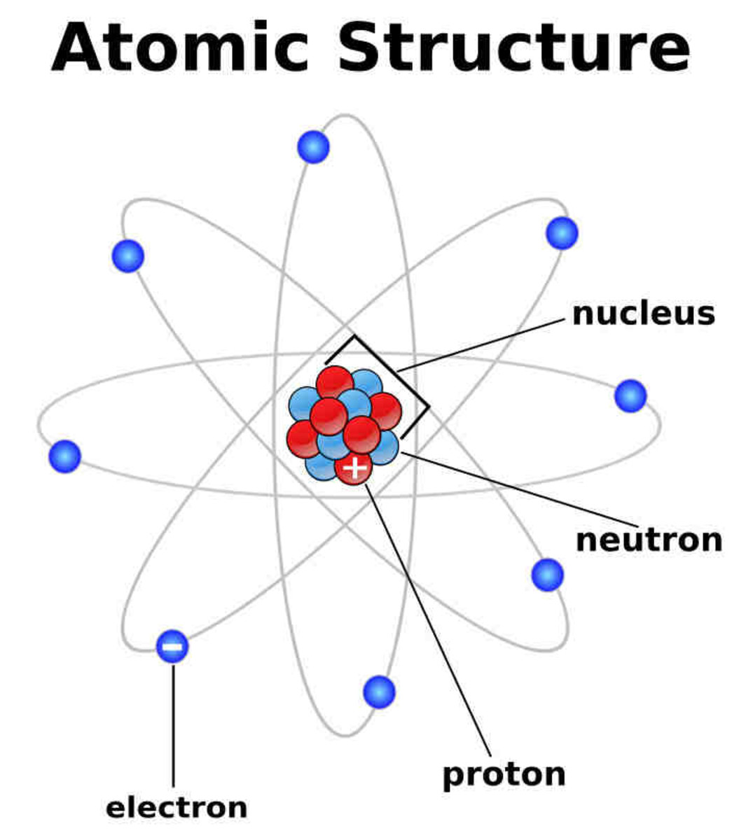
Carbon is a fundamental chemical element with a unique atomic structure that underpins its role as the backbone of organic chemistry and life on Earth. Its atomic number, 6, directly influences its electron configuration, bonding behavior, and placement in Group 14 (Carbon Group) of the periodic table. This configuration enables carbon to form stable covalent bonds with up to four other atoms, facilitating the vast diversity of organic compounds, from simple hydrocarbons to complex biomolecules like DNA and proteins.The atomic number of an element defines its identity by specifying the number of protons in its nucleus, which in turn determines the number of electrons in a neutral atom. For carbon, this means six protons and six electrons, arranged in a 1s² 2s² 2p² electron configuration. This arrangement allows carbon to achieve a stable octet by sharing electrons, a principle central to organic chemistry. The element’s small atomic size and high electronegativity further enhance its reactivity, enabling it to bond with elements like hydrogen, oxygen, and nitrogen to form the molecular building blocks of life.
Atomic Structure and Electron Configuration of Carbon
The atomic structure of carbon is defined by its proton count (6), which dictates its position in the periodic table and its chemical properties. The nucleus contains six protons and typically six neutrons (though isotopes like carbon-14 have variations), while the electron cloud consists of two electron shells:This configuration, particularly the presence of four valence electrons (2s² 2p²), allows carbon to form four covalent bonds through sp³ hybridization, a process that explains its tetrahedral geometry in methane (CH₄) and other organic molecules. The ability to form single, double, and triple bonds (e.g., in alkenes like ethylene or alkynes like acetylene) further expands carbon’s versatility in molecular structures.
Key Formula:
The electron configuration of carbon in its ground state:
1s² 2s² 2p²
Valence electrons: 4 (2s² 2p²)
Chemical Behavior and Bonding Capabilities Determined by Atomic Number 6
The atomic number of carbon (6) directly influences its chemical behavior by dictating its valence electron count and bonding capacity. With four valence electrons, carbon exhibits:These properties stem from carbon’s position in Group 14, where elements share a tendency to form four bonds. However, carbon’s small atomic radius and high bond dissociation energy make its bonds particularly stable. For example, the C–C single bond has a bond energy of 347 kJ/mol, while the C=O double bond in carbonyl groups is 799 kJ/mol, illustrating the strength and diversity of carbon-based bonding.
Comparison of Carbon with Adjacent Elements in the Periodic Table
Carbon’s properties can be contrasted with those of neighboring elements in Period 2 (Nitrogen, Oxygen) and Group 14 (Silicon), highlighting how its atomic number (6) positions it uniquely for organic chemistry.| Element Name | Atomic Number | Key Characteristics |
|---|---|---|
| Carbon (C) | 6 |
|
| Nitrogen (N) | 7 |
|
| Oxygen (O) | 8 |
|
| Hydrogen (H) | 1 |
|
| Silicon (Si) | 14 |
|
Locating Carbon’s Atomic Number Using a Standard Periodic Table
The periodic table organizes elements by increasing atomic number, with carbon positioned in Period 2, Group 14. To locate carbon’s atomic number (6) using a standard layout, follow this step-by-step procedure:1. Identify the Periods (Rows):
Historical Context and Discovery of Carbon’s Atomic Number
The determination of carbon’s atomic number (Z = 6) represents a pivotal milestone in the evolution of atomic theory and the periodic table. Early atomic models, from Dalton’s indivisible atoms to Rutherford’s nuclear structure, laid the groundwork for understanding subatomic particles, while advancements in spectroscopy—particularly X-ray analysis—provided the empirical tools to quantify proton counts. The formalization of atomic numbers as defining elements, rather than atomic weights, emerged through collaborative efforts spanning the late 19th and early 20th centuries, with key contributions from Dmitri Mendeleev, Henry Moseley, and others. This subtopic examines the scientific milestones, theoretical frameworks, and experimental techniques that culminated in the precise identification of carbon’s atomic number, emphasizing the interplay between theory and observation.Early Atomic Theories and the Foundations of Atomic Number Conceptualization
Prior to the 20th century, atomic theory lacked a mechanistic framework to distinguish elements beyond their relative atomic masses. John Dalton’s 1803 atomic theory posited that elements consisted of indivisible particles, but it offered no means to differentiate between atoms of varying proton counts. The discovery of electrons by J.J. Thomson in 1897 (via cathode ray experiments) introduced the concept of subatomic structure, suggesting atoms were composite rather than fundamental. Thomson’s "plum pudding" model proposed a positively charged matrix with embedded electrons, yet it failed to account for atomic diversity or the role of protons. Ernest Rutherford’s 1911 gold foil experiment revolutionized atomic theory by revealing a dense, positively charged nucleus, implying that atomic properties—including identity—were governed by nuclear composition. This shift from mass-based to charge-based differentiation set the stage for atomic numbers as the defining characteristic of elements.The transition from atomic weight to atomic number as the organizing principle of the periodic table was crystallized by Henry Moseley’s 1913 work on X-ray spectroscopy. Moseley demonstrated that the frequency of characteristic X-ray emissions from an element correlated directly with the square root of its nuclear charge (Z), formalizing the relationship:
√f = a(Z − b)This empirical law provided the first quantitative method to assign atomic numbers, resolving ambiguities in Mendeleev’s periodic table (e.g., the placement of tellurium and iodine) and confirming carbon’s position as Z = 6.
where f is the frequency of the Kα X-ray line, a and b are constants, and Z is the atomic number.
Key Milestones in the Identification of Carbon’s Atomic Number
The progression toward carbon’s atomic number was marked by four critical developments, each addressing gaps in atomic theory or experimental technique. These milestones reflect the cumulative nature of scientific discovery, where theoretical insights and technological innovations converged to redefine elemental classification.The timeline below highlights the foundational events:
-
1869: Mendeleev’s Periodic Table and the Atomic Weight Paradox
Dmitri Mendeleev’s arrangement of elements by increasing atomic weight revealed periodic trends but included inconsistencies, such as the reversal of tellurium (Te) and iodine (I). His predictive power—anticipating undiscovered elements like germanium—demonstrated the need for a more fundamental organizing principle. Carbon, with an atomic weight of ~12, was placed early in Group IV but lacked a mechanism to distinguish it from other light elements like nitrogen (N) or boron (B). -
1911: Rutherford’s Nuclear Model and the Proton’s Role
Rutherford’s discovery of the atomic nucleus established that an element’s identity depended on its nuclear charge, not merely mass. While protons were not yet isolated (their existence was inferred from hydrogen’s nucleus), this model implied that atomic numbers—representing proton counts—would uniquely define elements. Carbon’s position as Z = 6 was inferred from its spectral properties and relative placement in the periodic table, though direct confirmation awaited spectroscopic advancements. -
1913: Moseley’s X-Ray Spectroscopy and the Atomic Number Scale
Moseley’s experiments on X-ray emission spectra provided the decisive link between nuclear charge and atomic identity. By bombarding elements with electrons and measuring the resulting X-ray frequencies, he derived a linear relationship between Z and spectral lines. For carbon, the Kα line (a transition in the innermost electron shell) corresponded to Z = 6, aligning with its position in the periodic table and resolving earlier ambiguities. This work also exposed flaws in atomic weight-based ordering, as elements like argon (Z = 18) and potassium (Z = 19) were correctly positioned despite their inverted weights. -
1920s–1930s: Neutron Discovery and the Completion of Atomic Structure
The identification of neutrons by James Chadwick in 1932 confirmed that atomic mass exceeded nuclear charge due to neutron contributions. While neutrons did not affect atomic numbers, this discovery solidified the proton’s role as the defining particle of an element. Carbon’s atomic number remained Z = 6, with its most abundant isotope (¹²C) comprising 6 protons and 6 neutrons, serving as the standard for atomic mass units (u) in the modern metric system.
Spectroscopy’s Role in Confirming Carbon’s Atomic Number
Spectroscopy emerged as the definitive tool for assigning atomic numbers, leveraging the quantized energy transitions of electrons in atomic orbitals. The relationship between spectral lines and nuclear charge is rooted in Bohr’s atomic model (1913), which posited that electrons occupy discrete energy levels and emit or absorb radiation when transitioning between them. For carbon, the Kα X-ray line—produced when an outer electron fills a vacancy in the K-shell (n=1)—is particularly diagnostic.Moseley’s law established that the frequency (f) of this line scales with Z², allowing precise determination of proton counts. For carbon, the Kα line occurs at approximately 0.0282 Å (angstroms), corresponding to a frequency of ~3.0 × 10¹⁸ Hz. This value aligns with Z = 6 when substituted into Moseley’s equation, confirming carbon’s nuclear charge. The consistency of this relationship across elements validated the atomic number as the fundamental property of an element, superseding atomic weight as the organizing principle of the periodic table.
The significance of spectroscopy extended beyond carbon: it provided a method to discover new elements (e.g., hafnium, Z = 72, identified in 1923 via X-ray spectra) and resolve discrepancies in Mendeleev’s table. For carbon specifically, spectroscopic confirmation aligned with its chemical behavior—such as forming four covalent bonds—and its position as the backbone of organic chemistry. The stability of carbon’s atomic number (unlike its isotopes, which vary in neutron count) underscores the proton’s invariant role in defining elemental identity.
:max_bytes(150000):strip_icc()/atomic-structure-conceptual-artwork-99312661-58af58c75f9b5860467ff472.jpg)
Applications of Carbon’s Atomic Number in Chemistry
Carbon’s atomic number (6) defines its electronic configuration (1s² 2s² 2p²), enabling it to form four covalent bonds through sp³, sp², and sp hybridization. This versatility distinguishes carbon from neighboring elements in the periodic table, influencing reactivity, bonding diversity, and the foundation of organic chemistry. While boron (atomic number 5) and nitrogen (atomic number 7) exhibit limited bonding capabilities due to their electron deficiencies or excesses, carbon’s tetravalency and ability to catenate (bond with itself) create unparalleled structural complexity. The following analysis compares carbon’s reactivity with boron and nitrogen, explores its role as the backbone of organic molecules, and examines how its atomic properties facilitate life’s molecular architecture.Comparative Reactivity of Carbon with Boron and Nitrogen
The bonding behavior of carbon, boron, and nitrogen is fundamentally shaped by their atomic numbers, which determine valence electrons and bonding capacity. Carbon’s four valence electrons allow it to form stable covalent bonds with hydrogen, oxygen, and other carbon atoms, whereas boron’s three valence electrons result in electron-deficient bonding (e.g., Lewis acids), and nitrogen’s five valence electrons lead to lone-pair-driven reactivity (e.g., basicity). The following table summarizes key differences in bonding types and common compounds formed by these elements:| Element | Atomic Number | Bonding Type | Common Compounds |
|---|---|---|---|
| Boron | 5 |
|
|
| Carbon | 6 |
|
|
| Nitrogen | 7 |
|
|
Carbon’s Atomic Number and the Foundation of Organic Chemistry
The atomic number 6 endows carbon with tetravalency and catenation, two properties that make it the central element of organic molecules. Unlike boron (which rarely forms extended structures) or nitrogen (which primarily participates in small, functionalized groups), carbon atoms can bond to one another in linear chains, branched networks, and cyclic rings, creating the diversity of organic compounds essential for life. This versatility is governed by hybridization rules:- sp³ Hybridization: Tetrahedral geometry (e.g., methane, CH₄; ethane, C₂H₆).
Molecular Structure Examples and Formation Rules:
Organic molecules are built from carbon backbones adorned with functional groups. For instance:
The octet rule and valence shell electron pair repulsion (VSEPR) theory further explain why carbon’s four bonds are geometrically optimized for stability. Unlike boron (which often violates the octet rule) or nitrogen (which frequently forms lone pairs), carbon’s four bonds allow it to satisfy the octet while enabling modular assembly of larger molecules.
Flowchart: From Atomic Number to Molecular Complexity
The progression from carbon’s atomic number (6) to its role in forming life’s macromolecules can be visualized as follows:1. Electronic Configuration (1s² 2s² 2p²):
2. Covalent Bonding and Catenation:
3. Functional Group Attachment:
4. Macromolecular Assembly:
5. Emergent Properties:
Carbon’s atomic number (6) is the molecular architect of life’s diversity because it combines tetravalency, catenCarbon Isotopes and Variations in Atomic Mass
Carbon exhibits three naturally occurring isotopes—¹²C, ¹³C, and ¹⁴C—each characterized by a distinct atomic mass while retaining the same atomic number (6). This constancy of atomic number (protons) contrasts with variations in mass number (protons + neutrons), which arise from differing neutron counts. The stability and applications of these isotopes span from foundational chemistry to radiometric dating, with their unique properties enabling precise scientific measurements and historical reconstructions.The atomic number of carbon remains invariant across its isotopes due to the fixed number of protons (6) defining its elemental identity. However, the mass number varies due to additional neutrons: ¹²C contains 6 neutrons, ¹³C contains 7, and ¹⁴C contains 8. This variation influences nuclear stability, decay processes, and practical utility in fields such as archaeology, geology, and isotopic analysis.
Stability and Applications of Carbon Isotopes
The three isotopes of carbon exhibit distinct stability and functional roles, each exploited in scientific and industrial contexts:
- ¹²C (Carbon-12) serves as the standard reference for atomic mass units (u), defining 1/12th of its mass as the baseline for the unified atomic mass scale. Its abundance (98.93% of natural carbon) and stability make it indispensable in mass spectrometry, organic synthesis, and nuclear physics. The isotope’s uniformity in mass facilitates precise calibration of analytical instruments and theoretical calculations in quantum chemistry.
- ¹³C (Carbon-13), comprising 1.07% of natural carbon, is a stable but less abundant isotope with a mass excess of +7.016 MeV relative to ¹²C. Its presence is critical in nuclear magnetic resonance (NMR) spectroscopy, where ¹³C NMR spectra reveal molecular structures by detecting nuclear spin transitions. Additionally, ¹³C isotopic ratios in biological samples provide insights into metabolic pathways and dietary studies, as plants discriminate against ¹³C during photosynthesis.
- ¹⁴C (Carbon-14) is a radioactive isotope with a half-life of 5,730 ± 40 years, formed in the upper atmosphere via cosmic ray spallation of nitrogen-14. Its decay via beta emission (β⁻) to nitrogen-14 enables radiocarbon dating, a cornerstone of archaeology and paleoclimatology. The isotope’s production rate remains relatively constant, allowing scientists to estimate the age of organic materials up to ~50,000 years. Industrial applications include tracing carbon flow in ecosystems and monitoring nuclear waste.
Mass Spectrometry and Isotope Discrimination
Mass spectrometry distinguishes carbon isotopes by leveraging differences in atomic mass while confirming the atomic number through ionization and magnetic deflection. The process begins with ionization, where carbon atoms are vaporized and bombarded with electrons, stripping them of electrons to form positively charged ions (typically C⁺). These ions are then accelerated through an electric field into a magnetic sector, where their trajectories deflect based on mass-to-charge ratio (m/z).
Key Principle: Lighter isotopes (e.g., ¹²C⁺) deflect more sharply than heavier isotopes (e.g., ¹⁴C⁺) under identical magnetic fields, enabling separation and detection via a Faraday cup or secondary electron multiplier.The resulting mass spectrum displays peaks corresponding to each isotope’s m/z value, with relative intensities reflecting natural abundances. For example, a sample’s ¹³C/¹²C ratio can be quantified by comparing peak heights at m/z 13 and 12, corrected for instrumental biases. This method underpins isotopic analysis in climate science, forensics, and pharmaceutical research, where precise mass discrimination is critical.
Comparative Properties of Carbon Isotopes
The following table summarizes the fundamental properties of carbon isotopes, including atomic mass and half-life where applicable:
Notes:
Isotope Atomic Mass (u) Half-Life ¹²C 12.000000 (exact, by definition) Stable (infinite half-life) ¹³C 13.0033548378(10) Stable (infinite half-life) ¹⁴C 14.003241989(15) 5,730 ± 40 years
Atomic masses are rounded to 5–6 decimal places for clarity; precise values are derived from IUPAC recommendations. The half-life of ¹⁴C is used for radiocarbon dating, with corrections applied for isotopic fractionation in samples. Natural abundance ratios: ¹²C (98.93%), ¹³C (1.07%), ¹⁴C (trace, ~10⁻¹²%).
Carbon in Modern Technology and Industry
The atomic number of carbon (6), defining its electron configuration and bonding capabilities, underpins its dominance in materials science and industrial applications. Carbon’s ability to form stable covalent bonds—whether in sp³ (diamond), sp² (graphene), or sp (carbon nanotubes) hybridizations—directly influences its mechanical, electrical, and thermal properties. These atomic-scale characteristics enable carbon-based materials to outperform traditional counterparts in strength, conductivity, and lightweight structural integrity. The versatility of carbon’s bonding network extends beyond pure elemental forms, facilitating composites and hybrid structures critical in aerospace, energy storage, and advanced manufacturing.
Atomic Structure and Material Innovations
Carbon’s atomic number dictates its bonding behavior, which is exploited in engineered materials with tailored properties. Graphene, a single atomic layer of sp²-hybridized carbon arranged in a hexagonal lattice, exhibits exceptional electrical conductivity (up to 10⁶ S/m) and tensile strength (130 GPa) due to delocalized π-electrons and strong σ-bonds. Its atomic thickness (0.335 nm) enables applications in transparent conductive films and quantum electronics. Diamond, composed of sp³-hybridized carbon atoms in a tetrahedral lattice, achieves hardness (10 on the Mohs scale) and thermal conductivity (2,000 W/m·K) through dense 3D covalent networks. Carbon fibers, synthesized via controlled pyrolysis of polyacrylonitrile (PAN) or pitch, retain sp²-rich graphitic structures along their axes, providing high stiffness-to-weight ratios (modulus up to 700 GPa) for aerospace and automotive composites.The atomic number also governs carbon nanotubes (CNTs), cylindrical structures with sp²-bonded carbon atoms forming seamless tubes. Single-walled CNTs (SWCNTs) exhibit diameters of ~1 nm and aspect ratios exceeding 1,000:1, while multi-walled CNTs (MWCNTs) combine concentric tubes for enhanced mechanical reinforcement. Their electronic properties range from metallic to semiconducting, depending on chiral angles (e.g., armchair vs. zigzag configurations), enabling applications in field-effect transistors and energy storage.
Synthesis of Carbon-Based Nanomaterials: A Chemical Perspective
The atomic number of carbon (6) influences synthesis pathways by determining reaction stoichiometry, bonding energetics, and precursor decomposition. Below is a step-by-step outline for synthesizing carbon nanotubes (CNTs) via chemical vapor deposition (CVD), emphasizing atomic-level interactions:1. Precursor Selection and Activation
Carbon sources such as methane (CH₄), ethylene (C₂H₄), or ethanol (C₂H₅OH) are introduced into a reactor at 700–1,200°C. The atomic number of carbon (6) ensures that each precursor molecule can decompose into atomic or molecular carbon fragments (e.g., CH₃ radicals) without requiring excessive energy, due to the stability of C–C bonds (bond dissociation energy: ~347 kJ/mol). Transition metals (Fe, Co, Ni) catalyze decomposition by lowering the activation energy for C–C bond formation.2. Nucleation and Growth
Carbon atoms dissolve into metal nanoparticles, supersaturating the lattice and precipitating as graphene layers. The atomic number dictates the carbon solubility limit in metals (e.g., ~10 at% in Fe at 1,000°C), influencing nucleation rates. Growth occurs via base growth (catalyst anchored to substrate) or tip growth (catalyst particle detaches), with sp² hybridization stabilizing the tubular structure. The chiral angle (θ) of the nanotube is determined by the ratio of precursor carbon atoms to catalyst sites, where θ = arctan(√3 n/(m + n)) for (n,m) indices.3. Post-Growth Functionalization
CNTs undergo oxidation (e.g., H₂SO₄/HNO₃) to introduce carboxyl (–COOH) or hydroxyl (–OH) groups, leveraging carbon’s ability to form stable C–O bonds. This step enables covalent or non-covalent functionalization for targeted applications, such as polymer composites or biosensors. The atomic number ensures compatibility with organic chemistries, as carbon’s electronegativity (2.55) facilitates polar interactions.
Carbon’s Role in Energy Storage Systems
The atomic number of carbon enables its integration into high-performance energy storage devices, particularly in lithium-ion batteries (LIBs), where it serves as an anode material or conductive framework. Carbon’s lightweight atomic mass (12.01 g/mol) and high electrical conductivity (graphite: ~10⁴ S/m) reduce system weight while maintaining charge transport efficiency. In graphite anodes, lithium intercalates between graphene layers (sp²-bonded carbon) during discharge, forming LiC₆ with a theoretical capacity of 372 mAh/g. The atomic structure of graphite (layer spacing: 0.335 nm) accommodates lithium ions without collapsing, unlike silicon anodes (which expand by ~400%).For silicon-carbon composites, amorphous carbon coatings (sp³-hybridized) encapsulate silicon nanoparticles, mitigating volume expansion during lithiation. The atomic number ensures carbon’s inertness toward lithium (no alloying), while its conductive network stabilizes electron transport. In supercapacitors, activated carbon (high surface area: 1,000–3,000 m²/g) exploits sp²-rich porosity for electrostatic double-layer capacitance, achieving energy densities up to 10 Wh/kg.
Industrial Applications Leveraging Carbon’s Atomic Number
Carbon’s atomic properties are pivotal in industries where material performance, durability, and functional versatility are critical. Below are four sectors where carbon’s atomic number (6) enables transformative applications:
Key Principle: The atomic number of carbon (6) ensures four valence electrons, facilitating covalent bonding in diverse hybridizations (sp³, sp², sp) and enabling tunable material properties.
- Aerospace and Defense
Carbon fibers, synthesized via controlled pyrolysis of PAN or mesophase pitch, retain sp²-rich graphitic structures that provide specific tensile strength (strength-to-weight ratio) exceeding 1,800 kN·m/kg. In Boeing 787 Dreamliner, carbon fiber-reinforced polymers (CFRP) reduce structural weight by 20% compared to aluminum, improving fuel efficiency. The atomic number ensures carbon’s lightweight atomic mass (12.01 g/mol) while maintaining stiffness (modulus up to 700 GPa), critical for aircraft wings and fuselage components.- Electronics and Semiconductors
Graphene’s atomic-scale thickness (0.335 nm) and high electron mobility (200,000 cm²/V·s) enable transparent conductive films for touchscreens and flexible displays. In RFID tags, graphene replaces indium tin oxide (ITO) due to its conductivity and mechanical flexibility. The atomic number’s influence on sp² hybridization allows for tunable bandgaps in graphene nanoribbons (GNRs), enabling applications in quantum computing and high-frequency transistors.- Pharmaceuticals and Drug Delivery
Carbon nanotubes (CNTs) exploit their atomic structure for targeted drug delivery, where functionalized SWCNTs (diameter: ~1 nm) penetrate cell membranes via endocytosis. The atomic number facilitates covalent attachment of therapeutic molecules (e.g., doxorubicin) to CNT sidewalls, enabling controlled release triggered by pH or enzymatic activity. In cancer therapy, MWCNTs (multi-walled) serve as photothermal agents, converting near-infrared light into heat due to their sp²-bonded graphitic layers.- Energy and Environmental Technologies
Activated carbon (porous sp²-hybridized carbon) removes contaminants (e.g., arsenic, PFAS) via adsorption, with surface areas exceeding 2,500 m²/g. The atomic number ensures carbon’s non-toxicity and chemical stability, critical for water purification systems. In CO₂ capture, carbon-based sorbents (e.g., metal-organic frameworks with carbon linkers) leverage sp² hybridization to enhance CO₂ affinity (binding energy: ~25 kJ/mol) while resisting degradation in harsh conditions.Carbon’s atomic number of six is more than a numerical identifier; it is the blueprint for molecular diversity, technological advancement, and biological existence. From the precision of radiocarbon dating to the strength of carbon fibers in aerospace engineering, this fundamental property illustrates the profound interplay between atomic structure and real-world impact. As research continues to harness carbon’s unique capabilities—whether in nanotechnology or sustainable energy—its atomic number remains a testament to the elegance of chemistry and the boundless potential of scientific discovery.
FAQ
What is the atomic number of carbon dioxide (CO₂)?
Carbon dioxide (CO₂) contains one carbon atom and two oxygen atoms. The atomic number of carbon is 6, and oxygen’s is 8, but CO₂ itself doesn’t have a single atomic number—it’s a molecule. The atomic number refers only to individual elements, not compounds.
What is the atomic number of carbon-14?
Carbon-14 is an isotope of carbon, meaning it has the same atomic number as all carbon atoms, which is 6. The "14" refers to its mass number (6 protons + 8 neutrons). The atomic number is determined by the number of protons, not neutrons.
What is the atomic number of carbon-13?
Carbon-13 is an isotope of carbon with an atomic number of 6, just like all carbon atoms. The "13" indicates its mass number (6 protons + 7 neutrons). The atomic number remains unchanged for any carbon isotope.
What is the atomic number of carbon-12?
The atomic number of carbon-12 is 6, as it has 6 protons in its nucleus. The "12" refers to its mass number (6 protons + 6 neutrons). Carbon-12 is the most common isotope and serves as the basis for the atomic mass unit (amu).
What are the atomic numbers of carbon and oxygen?
Carbon has an atomic number of 6, while oxygen has an atomic number of 8. These numbers represent the count of protons in each element’s nucleus.
What are the atomic numbers of carbon, magnesium, and lithium?
Carbon has an atomic number of 6, magnesium has 12, and lithium has 3. These values indicate the number of protons in each element’s nucleus.

Leave a Comment
Comments are moderated before appearing. The data you submit is processed according to the Privacy Policy of Voltefac.