What Is The Bohr Rutherford Model Explained Fundamentally
Table of Contents
- Historical Development and Key Contributors to the Bohr-Rutherford Model
- Preceding Atomic Theories and Their Limitations
- Rutherford’s Nuclear Model and the Gold Foil Experiment
- Bohr’s Modifications: Quantization and Electron Orbits
- Comparison: Rutherford’s Nuclear Model vs. Bohr’s Atomic Model
- Scientific Context and Theoretical Influences
- Core Principles and Structural Components of the Bohr-Rutherford Model
- Fundamental Assumptions of the Bohr-Rutherford Model
- Structural Components and Their Significance
- Mechanisms of Atomic Stability in the Bohr-Rutherford Model
- Electron Configuration and Energy Levels in the Bohr-Rutherford Model
- Rules Governing Electron Placement in Shells and Subshells
- Comparison of Electron Configurations for Hydrogen, Helium, and Lithium
- Limitations in Predicting Electron Transitions Beyond Hydrogen
- Applications and Practical Examples of the Bohr-Rutherford Model
- Pedagogical Value in Modern Education
- Historical Experiments Validating or Challenging the Model
- Simulating the Bohr Model: A Planetary Analogy Procedure
- Visual Representations and Analogies of the Bohr-Rutherford Model
- Text-Based Visualizations of Hydrogen and Helium Atoms
- Analogies for Electron Behavior in the Bohr-Rutherford Model
- Evolution of Textbook Depictions: From Planetary to Orbital Models
- Common Misconceptions in Visual Representations
- Criticisms and Evolution into Modern Theories
- Experimental Failures and Quantum Mechanical Corrections
- Comparison of Electron Descriptions: Bohr-Rutherford vs. Schrödinger Wavefunctions
- Contributions of Later Scientists to Atomic Theory
- FAQ
- what is the ernest rutherford model?
- what is the bohr rutherford diagram?
- what is the bohr rutherford diagram for hydrogen?
- what is the bohr rutherford diagram for magnesium?
- what is the bohr rutherford diagram for lithium?
- what is the bohr rutherford diagram for carbon?
The Bohr-Rutherford model revolutionized atomic theory by introducing a structured framework that merged Ernest Rutherford’s nuclear discovery with Niels Bohr’s quantized electron orbits. Emerging in the early 20th century, this model shifted scientific understanding from Thomson’s diffuse "plum pudding" atom to a precise, layered atomic architecture. Its foundational principles—fixed electron paths and discrete energy levels—provided the first coherent explanation for atomic stability and spectral line patterns, bridging classical physics with nascent quantum mechanics.
Rooted in Rutherford’s 1911 gold foil experiment, which exposed the nucleus as a dense, positively charged core, Bohr’s 1913 modifications introduced revolutionary concepts: electrons occupy quantized orbits where angular momentum is an integer multiple of h/2π, and transitions between levels emit or absorb energy as photons. This paradigm not only resolved inconsistencies in atomic behavior but also laid the groundwork for later quantum theories, despite its eventual limitations in multi-electron systems. The model’s enduring legacy lies in its pedagogical clarity and historical significance as a transitional theory in atomic physics.

Historical Development and Key Contributors to the Bohr-Rutherford Model
The Bohr-Rutherford model emerged as a pivotal advancement in atomic theory during the early 20th century, synthesizing experimental evidence with theoretical refinements. Ernest Rutherford’s groundbreaking nuclear model (1911) established the atomic nucleus, while Niels Bohr’s modifications (1913) introduced quantized electron orbits, resolving inconsistencies in classical physics. This section explores the chronological progression of atomic theories, the foundational experiments of Rutherford and Bohr, and their collaborative refinement of the atomic structure model.
Preceding Atomic Theories and Their Limitations
Before the Bohr-Rutherford model, atomic theory was shaped by earlier hypotheses that sought to explain the composition of matter. The Daltonian atomic theory (1803) proposed atoms as indivisible, solid spheres with uniform mass, lacking internal structure. This model successfully explained chemical reactions but failed to account for subatomic particles or atomic spectra.
The Thomson’s plum pudding model (1897) introduced electrons as negatively charged particles embedded in a positively charged "pudding" of matter, derived from cathode ray experiments. While this model explained electron discovery, it could not reconcile the stability of atoms or the results of subsequent scattering experiments.
These limitations underscored the need for a model that incorporated nuclear charge concentration and electron behavior, directly influencing Rutherford’s and Bohr’s contributions.
Rutherford’s Nuclear Model and the Gold Foil Experiment
Ernest Rutherford’s nuclear model (1911) was primarily derived from the gold foil experiment (1909–1910), conducted by Hans Geiger and Ernest Marsden under his supervision. The experiment involved firing alpha particles (helium nuclei) at a thin gold foil and observing their deflection patterns.Key observations included:
Rutherford’s conclusions challenged Thomson’s model by proposing:
Rutherford’s Nuclear Model Assumptions:
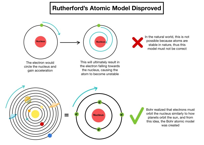
Electrons move in random orbits around the nucleus. The nucleus contains protons (later confirmed with proton discovery in 1919). Atomic stability was unexplained, as classical physics predicted electrons would radiate energy and spiral into the nucleus.
Bohr’s Modifications: Quantization and Electron Orbits
Niels Bohr’s 1913 model addressed the instability issue in Rutherford’s atomic structure by incorporating quantum theory, specifically Max Planck’s quantization of energy and Einstein’s photoelectric effect. Bohr’s key contributions included:- Quantized Electron Orbits: Electrons occupy discrete, stable orbits with fixed energies, corresponding to specific radii. These orbits are labeled by the principal quantum number (n).
Bohr’s model successfully explained the hydrogen emission spectrum, where electrons transitioning between energy levels emit light at specific wavelengths (e.g., the Balmer series). However, it was limited to single-electron systems and failed to account for multi-electron atoms or fine spectral details.
Comparison: Rutherford’s Nuclear Model vs. Bohr’s Atomic Model
The following table contrasts the foundational differences between Rutherford’s nuclear model and Bohr’s quantized atomic model, emphasizing electron behavior, structural assumptions, and theoretical innovations.| Feature | Rutherford’s Nuclear Model (1911) | Bohr’s Atomic Model (1913) |
|---|---|---|
| Electron Orbits | Random, non-quantized paths; classical mechanics applied. | Discrete, quantized orbits with fixed energies (n = 1, 2, 3...). |
| Atomic Stability | Unstable; electrons should spiral into the nucleus (classical prediction). | Stable; electrons in ground states do not radiate energy. |
| Energy Levels | Not addressed; continuous energy spectrum assumed. | Quantized energy levels; transitions emit/absorb photons. |
| Experimental Basis | Gold foil scattering experiment (alpha particle deflection). | Hydrogen emission spectrum (Balmer series) and Planck’s quantum theory. |
| Nuclear Composition | Protons only (neutrons undiscovered; mass discrepancy noted). | Protons and neutrons (later incorporated post-1932). |
| Applicability | General atomic structure; no spectral predictions. | Successful for hydrogen; limited to single-electron systems. |
Scientific Context and Theoretical Influences
The development of the Bohr-Rutherford model was deeply rooted in the electromagnetic and quantum revolutions of the late 19th and early 20th centuries. Key influences included:- Classical Electrodynamics (Maxwell): Predicted that accelerating charged particles (e.g., electrons in orbits) would emit radiation, leading to atomic instability. This conflict necessitated Bohr’s quantization.
where R is the Rydberg constant (1.097 × 10⁷ m−1), and n1, n2 are quantum numbers. The synthesis of these ideas bridged experimental observations with theoretical innovation, laying the groundwork for modern quantum mechanics. While the Bohr-Rutherford model was later superseded by Schrödinger’s wave mechanics (1926) and Heisenberg’s uncertainty principle (1927), its foundational role in atomic theory remains indispensable.
Core Principles and Structural Components of the Bohr-Rutherford Model
The Bohr-Rutherford model revolutionized atomic theory by introducing discrete electron orbits and quantized energy levels, addressing critical gaps in Rutherford’s nuclear model. This framework combined empirical observations with mathematical precision, establishing a foundational understanding of atomic structure that bridged classical physics with early quantum mechanics. The model’s core principles—fixed electron trajectories, energy quantization, and the role of the nucleus—provided a stable yet dynamic representation of atomic behavior, influencing later developments in spectroscopy and chemical bonding.The structural components of the model emphasize the nucleus as the dense, positively charged center, electron shells as quantized energy levels, and atomic numbers (Z) and mass numbers (A) as defining properties of elements. Below, the fundamental assumptions and their implications are explored, followed by a visual and conceptual breakdown of the model’s architecture and the mechanisms ensuring atomic stability.
Fundamental Assumptions of the Bohr-Rutherford Model
The Bohr-Rutherford model rests on three foundational assumptions that diverged from classical electromagnetic theory, which predicted that accelerating electrons should radiate energy and spiral into the nucleus. Niels Bohr’s modifications introduced stability through quantization, while Ernest Rutherford’s nuclear model provided the structural context.Key Assumptions:These assumptions resolved the "ultraviolet catastrophe" of classical physics by restricting electron motion to stable, non-radiative paths. The model’s success lay in its ability to explain hydrogen’s emission spectrum (Balmer series) and later extend to multi-electron atoms with modifications. However, it remained limited to single-electron systems due to its reliance on the Coulomb force and lack of consideration for electron-electron interactions.
1. Electrons occupy fixed, circular orbits around the nucleus without radiating energy, contradicting classical physics predictions.
2. Energy levels are quantized, meaning electrons can only exist in specific, discrete orbits corresponding to distinct energy values.
3. Electron transitions between orbits emit or absorb energy in the form of photons, with energy differences matching observed spectral lines.
4. The nucleus contains protons and (later confirmed) neutrons, with its positive charge balancing the negative charge of electrons to ensure atomic neutrality.
Structural Components and Their Significance
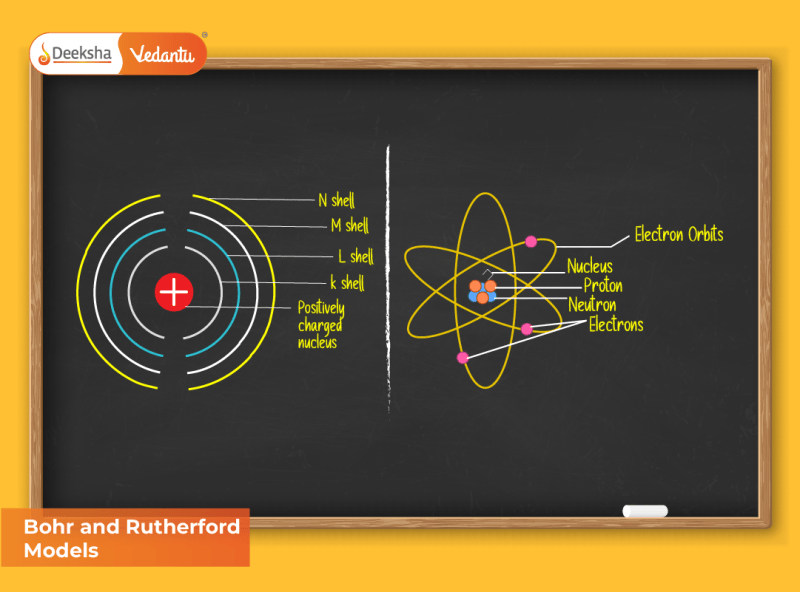
The Bohr-Rutherford model visualizes the atom as a miniature solar system, with the nucleus at the center and electrons orbiting in defined shells. Below is a conceptual breakdown of its components, emphasizing their roles in defining atomic identity and behavior.Visual Representation of the Model’s ComponentsThe atomic number (Z) uniquely identifies an element by specifying the number of protons, which dictates the number of electrons in a neutral atom. The mass number (A) accounts for nuclear composition, influencing the atom’s isotopic variants. For example, uranium-235 (Z=92, A=235) and uranium-238 (Z=92, A=238) share the same chemical properties but differ in nuclear stability and decay rates.Nucleus:Electron Shells:
- A dense central region containing protons (positive charge) and neutrons (neutral mass).
- Mass number (A) = protons (Z) + neutrons (N).
- Charge number (Z) determines the element’s identity (e.g., Z=1 for hydrogen, Z=6 for carbon).
Atomic Number (Z) and Mass Number (A):
- Discrete orbits (n=1, 2, 3...) corresponding to quantized energy levels.
- Shell capacity follows the 2n² rule (e.g., n=1 holds 2 electrons, n=2 holds 8).
- Electrons in higher shells have greater potential energy and are less tightly bound.
- Z (atomic number): Defines the element (e.g., helium has Z=2, with 2 protons and 2 electrons in a neutral state).
- A (mass number): Sum of protons and neutrons; isotopes differ in A but share Z (e.g., carbon-12 and carbon-14).
Mechanisms of Atomic Stability in the Bohr-Rutherford Model
Atomic stability in the Bohr-Rutherford model arises from a balance between two opposing forces: the electrostatic attraction between protons and electrons, and the centrifugal force (or centripetal acceleration) arising from electron motion. This equilibrium prevents electrons from collapsing into the nucleus while constraining them to quantized orbits.Force Balance in Electron OrbitsThe equilibrium condition derived from these forces leads to quantized orbital radii and energy levels, as described by Bohr’s postulates. For hydrogen (Z=1), the radius of the n orbit is given by:Electrostatic Attraction:Centrifugal Force (Centripetal Acceleration):
- Coulomb force between protons (positive) and electrons (negative) pulls electrons toward the nucleus.
- Magnitude: F = k·(Z·e²)/r², where k is Coulomb’s constant, e is electron charge, and r is orbital radius.
Equilibrium Condition:
- Electrons in circular motion experience an outward "centrifugal" effect balanced by the nucleus’s inward pull.
- Magnitude: F = m·v²/r, where m is electron mass and v is orbital velocity.
- For stability, electrostatic attraction equals centripetal force: k·(Z·e²)/r² = m·v²/r.
- Solving for velocity (v) yields quantized values dependent on the principal quantum number (n).
rₙ = (n²·ħ²)/(m·e²·k), where ħ is the reduced Planck constant.This relationship explains why electrons in hydrogen occupy discrete shells (e.g., the Bohr radius for n=1 is ~0.529 Å) and why transitions between shells (e.g., n=3 to n=2) emit specific wavelengths of light, as observed in emission spectra. The model’s stability condition also underscores why multi-electron atoms require adjustments (e.g., shielding effects in the Bohr-Sommerfeld model) to account for electron-electron repulsions.
Electron Configuration and Energy Levels in the Bohr-Rutherford Model
The Bohr-Rutherford model revolutionized atomic theory by introducing quantized electron orbits, but its application to electron configuration and energy levels remains constrained by its simplistic assumptions. While the model successfully explains hydrogen’s single-electron system, it struggles with multi-electron atoms due to electron-electron interactions and wave-like behavior. This section examines the rules governing electron placement within shells and subshells, compares configurations for hydrogen, helium, and lithium, and evaluates the model’s limitations in predicting transitions beyond hydrogen while highlighting its foundational role in quantum mechanics.The Bohr-Rutherford model treats electrons as particles in fixed orbits with discrete energy levels, governed by the principal quantum number n. Electron configuration follows empirical rules derived from experimental observations, such as the 2n² rule for maximum electrons per shell and the Pauli exclusion principle, which restricts electrons to unique quantum states. However, these rules were later refined by quantum mechanics, revealing discrepancies in multi-electron systems where electron-electron repulsion and orbital shapes (s, p, d, f) become critical. Despite its limitations, the model provided the conceptual framework for later theories, including Schrödinger’s wave mechanics, which introduced probabilistic electron distributions.
Rules Governing Electron Placement in Shells and Subshells
The Bohr-Rutherford model simplifies electron arrangement by assigning electrons to concentric shells (n = 1, 2, 3, ...) with energy levels proportional to n². Key principles include:- Shell Capacity (2n² Rule):
Each shell can accommodate a maximum of 2n² electrons, where n is the principal quantum number. For example:
- Pauli Exclusion Principle:
Enunciated by Wolfgang Pauli (1925), this principle states that no two electrons in an atom can occupy the same quantum state, defined by four quantum numbers: n, l (angular momentum), mₗ (magnetic), and ms (spin, ±½). The Bohr-Rutherford model implicitly enforces this by treating electrons as distinct particles in separate orbits, though it lacks the mathematical framework to describe spin or subshells.
- Aufbau Principle and Hund’s Rule:
While not explicitly part of the Bohr-Rutherford model, these principles were later applied to explain electron filling order. The Aufbau principle dictates that electrons occupy the lowest-energy orbitals first, and Hund’s rule specifies that electrons fill degenerate orbitals (same energy) singly before pairing. The Bohr model’s rigid shells do not account for orbital energies within subshells, leading to inaccuracies in predicting configurations for atoms beyond hydrogen.
Comparison of Electron Configurations for Hydrogen, Helium, and Lithium
The Bohr-Rutherford model’s electron configurations for the first three elements are summarized below, alongside modern quantum mechanical interpretations to highlight discrepancies.| Element | Atomic Number (Z) | Bohr-Rutherford Configuration | Modern Quantum Configuration | Discrepancies/Limitations |
|---|---|---|---|---|
| Hydrogen | 1 | 1s¹ (n=1, single electron) | 1s¹ | Accurate: Matches experimental spectra and energy levels. The model’s single-electron assumption aligns with quantum mechanics for hydrogen. |
| Helium | 2 | 1s² (n=1, two electrons) | 1s² | Partially Accurate: Correctly predicts 2 electrons in the K-shell but fails to explain helium’s stability beyond the 2n² rule. Quantum mechanics confirms the 1s² configuration but attributes stability to electron-electron repulsion and nuclear charge screening. |
| Lithium | 3 | 1s² 2s¹ (n=1 and n=2 shells) | 1s² 2s¹ | Limited Accuracy: Predicts the correct shell distribution but ignores subshell energies. Quantum mechanics reveals that the 2s orbital has lower energy than 2p, and the model cannot explain why lithium’s valence electron occupies 2s over 2p. Additionally, the model does not account for the shielding effect, where inner electrons reduce the effective nuclear charge felt by outer electrons. |
Limitations in Predicting Electron Transitions Beyond Hydrogen
The Bohr-Rutherford model’s success with hydrogen stems from its treatment of a single electron in a Coulomb potential, where energy levels are given by:Eₙ = −13.6 eV / n² (for hydrogen, where n is the principal quantum number).However, for multi-electron atoms, the model’s limitations become apparent:
- Electron-Electron Repulsion:
The model assumes electrons move independently in a fixed nuclear potential, ignoring inter-electron repulsion. In reality, electrons in multi-electron atoms experience shielding (reduced nuclear attraction due to inner electrons) and penetration (valence electrons spending time near the nucleus). This leads to energy level splitting within shells (e.g., 2s vs. 2p), which the Bohr model cannot explain. For example, lithium’s 2s electron has lower energy than 2p, contrary to the model’s prediction of degenerate shells.
- Failure to Explain Spectral Lines for Multi-Electron Atoms:
The Bohr model’s transitions between energy levels (ΔE = hν) work for hydrogen but fail for helium or lithium. Experimental spectra of these atoms show fine structure (splitting of spectral lines due to spin-orbit coupling) and hyperfine structure (nuclear interactions), phenomena absent in the Bohr model. Quantum mechanics resolves this by introducing quantum numbers (l, mₗ, ms) and wavefunctions, which describe electron probability distributions rather than fixed orbits.
- No Explanation for Subshells (s, p, d, f):
The Bohr model’s shells are one-dimensional (radius-dependent), whereas quantum mechanics introduces angular momentum quantum number (l), defining subshells with distinct shapes (spherical for l=0, dumbbell for l=1, etc.). The model cannot account for the Aufbau principle or Hund’s rule, which govern how electrons fill subshells in multi-electron atoms.
- Groundwork for Wave Mechanics:
Despite its flaws, the Bohr-Rutherford model laid critical foundations for quantum theory:
The transition from the Bohr-Rutherford model to modern quantum mechanics illustrates the evolution of atomic theory, where probabilistic wavefunctions replaced fixed orbits to accommodate the complexities of multi-electron systems and relativistic effects.
Applications and Practical Examples of the Bohr-Rutherford Model
The Bohr-Rutherford model, despite its limitations in fully explaining atomic behavior, remains a foundational teaching tool in introductory chemistry and physics. Its pedagogical value lies in simplifying complex quantum concepts for beginners while illustrating key principles such as quantized energy levels, electron transitions, and atomic structure. In practical applications, the model serves as an accessible framework for understanding spectroscopy, chemical bonding basics, and the behavior of hydrogen-like atoms. Though modern quantum mechanics has superseded its strict orbital mechanics, the Bohr-Rutherford model continues to provide intuitive analogies for visualizing atomic phenomena in educational settings and historical scientific experiments.
Pedagogical Value in Modern Education
The Bohr-Rutherford model is primarily taught in introductory chemistry and physics courses to:
Instructors often use the model to:
Historical Experiments Validating or Challenging the Model
Several experiments provided empirical support for or posed challenges to the Bohr-Rutherford model, shaping its development and refinement. Below are key experiments with observed patterns and their alignment with Bohr’s postulates.Context:
These experiments were critical in validating the idea of quantized energy levels and discrete spectral lines, which formed the core of Bohr’s atomic theory. While later experiments (e.g., the Stern-Gerlach experiment) revealed limitations, these foundational studies remain central to understanding atomic structure.
-
Hydrogen Emission Spectrum (Balmer Series, 1885)
Observed Pattern: Discrete spectral lines in the visible region (410–700 nm) when hydrogen gas is excited electrically.
Alignment with Bohr’s Model:
- Bohr explained these lines as transitions of electrons between specific energy levels (n = 3 → n = 2).
- The formula for wavelengths: \( \frac{1}{\lambda} = R \left( \frac{1}{n_1^2} - \frac{1}{n_2^2} \right) \),
- Confirmed the quantization of energy levels and the existence of a ground state (n = 1).
-
Franck-Hertz Experiment (1914)
Observed Pattern: Mercury atoms absorbed energy in discrete packets (4.9 eV) when bombarded with electrons, corresponding to excitation from the ground state to the first excited state.
Alignment with Bohr’s Model:
- Demonstrated that electrons in atoms can only occupy specific energy levels, supporting Bohr’s postulate of quantized orbits.
- Provided experimental evidence against classical physics’ continuous energy transfer.
-
Rutherford’s Gold Foil Experiment (1909)
Observed Pattern: Most alpha particles passed through gold foil undeflected, but some were scattered at large angles, indicating a dense, positively charged nucleus.
Alignment with Bohr’s Model:
- While Rutherford’s experiment suggested a nuclear structure, Bohr later integrated the nucleus into his model, proposing electrons orbiting a central positive charge.
- The model retained the planetary analogy but introduced quantized orbits to explain stability (classical physics predicted electrons would radiate energy and spiral into the nucleus).
-
Stark Effect (1913)
Observed Pattern: Spectral lines of hydrogen split into multiple components when subjected to a strong electric field.
Challenges to Bohr’s Model:
- The Stark effect suggested that electron orbits were not strictly circular or fixed in space, implying additional factors (e.g., electron spin, relativistic corrections) were needed.
- Later explained by quantum mechanics, this phenomenon highlighted the model’s limitations in accounting for external perturbations.
-
X-Ray Spectroscopy (Moseley’s Law, 1913)
Observed Pattern: The frequency of X-ray emissions from atoms increased with atomic number (Z), following a square-root relationship.
Alignment with Bohr’s Model:
- Confirmed the nuclear charge (Z) as a fundamental property determining electron energy levels.
- Supported the idea of hydrogen-like atoms (single-electron systems) but showed that multi-electron atoms required modifications (e.g., shielding effects).
where \( R \) is the Rydberg constant, and \( n_1, n_2 \) are integer energy levels.
Simulating the Bohr Model: A Planetary Analogy Procedure
The Bohr-Rutherford model can be metaphorically simulated using a planetary system analogy, where electrons are treated as planets orbiting a sun-like nucleus. This approach helps visualize key concepts such as quantized orbits, energy levels, and electron transitions. Below is a step-by-step procedure for creating a simplified analog.Context:
This simulation is purely educational and does not reflect the actual quantum nature of electrons. However, it effectively demonstrates the discrete energy levels and electron transitions central to Bohr’s theory.
-
Materials Required:
- A small, dense object (e.g., a marble or ball bearing) to represent the nucleus.
- Lightweight, connected rings or strings at fixed distances from the nucleus to represent electron orbits (energy levels).
- Colored beads or markers to denote electrons moving along the orbits.
- A light source (e.g., LED) to simulate photon emission/absorption during transitions.
-
Setting Up the Nucleus:
- Place the dense object (nucleus) at the center of a flat surface or a 3D frame.
- Label the nucleus with its atomic number (Z) (e.g., Z = 1 for hydrogen).
-
Defining Energy Levels (Orbits):
- Attach concentric rings or strings at increasing radii from the nucleus, labeled with principal quantum numbers (n = 1, 2, 3, ...).
- Ensure the distance between rings increases with n (e.g., n = 2 is twice as far as n = 1 in a simplified 2D model).
- Key Concept: Each orbit corresponds to a specific energy level \( E_n = -\frac{13.6 \text{ eV}}{n^2} \) for hydrogen.
-
Placing Electrons in Orbits:
- Position electrons (beads) on the lowest available orbit (n = 1 for hydrogen) to represent the ground state.
- For multi-electron atoms (e.g., helium), place up to 2 electrons in the n = 1 orbit (Pauli exclusion principle analogy).
-
Simulating Electron Excitation:
- Use an external energy source (e.g., heat or electrical discharge) to "excite" an electron, moving it to a higher orbit (n = 2, 3, etc.).
- Represent this as the electron "jumping" from a lower to a higher ring.
- Key Concept: Excitation requires energy equal to the difference between energy levels \( \Delta E = E_{n_f} - E_{n_i} \).
-
Demonstrating Photon Emission:
- When an excited electron returns to a lower orbit, activate the light source to simulate photon emission.
- The color of the light can correspond to the wavelength of the emitted photon (e.g., red for n = 3 → n = 2 in hydrogen).
- Key Concept: The energy of the photon matches the energy difference between levels \( E_{\text{photon}} = h\nu = E_{n_i} - E_{n_f} \).
-
Visualizing Spectral Lines:
- Record the "colors" (wavelengths) emitted during multiple transitions to create a simulated emission spectrum.
- Compare the pattern to real hydrogen spectra (e.g.,
- The nucleus contains 1 proton (p⁺) with a +1 charge.
- A single electron (e⁻) orbits in the n=1 energy level, maintaining a -1 charge.
- Neutrons are absent in the most common hydrogen isotope (protium).
- The nucleus contains 2 protons (p⁺, +2 total charge) and 2 neutrons (n⁰, neutral).
- Two electrons occupy the n=1 energy level, each with -1 charge.
- The model assumes electrons share the same orbit (later refined in quantum mechanics).
- Limitations: This implied continuous motion and deterministic paths, contradicting wave-particle duality and Heisenberg’s uncertainty principle.
- Modern Contrast: Electrons exhibit probabilistic distributions (orbitals) rather than fixed orbits, described by wavefunctions (ψ) in the Schrödinger equation.
- Limitations: Overemphasized wave-like behavior while ignoring particle properties (e.g., photoelectric effect).
- Modern Contrast: Electrons are delocalized probability clouds (orbitals) with quantized energy, not rigid waves.
- Classical View: Electrons jump between discrete orbits like planets changing orbits (e.g., hydrogen emission spectra).
- Quantum View: Transitions involve energy quantization without defined paths; electrons exist as superpositions until measured (collapse of the wavefunction).
- Features:
- Nucleus drawn as a central dot with protons and neutrons labeled.
- Electrons shown as dots or circles on concentric rings (energy levels).
- Example: Rutherford’s 1911 nuclear model combined with Bohr’s orbits (e.g., The Newer Alchemy by William Crookes, 1912).
- Pedagogical Role: Simplified atomic structure for non-specialists but misled about electron behavior.
- Features:
- Introduced electron clouds or probability regions (e.g., Heisenberg’s uncertainty principle).
- Textbooks like General Chemistry (1950s) used dotted regions to show electron density.
- Example: Linus Pauling’s The Nature of the Chemical Bond (1939) depicted orbitals as fuzzy clouds.
- Shift: Acknowledged wave-like properties but retained Bohr’s energy levels.
- Features:
- Phase diagrams and 3D probability plots (e.g., p-orbitals as dumbbells, d-orbitals as cloverleafs).
- Software tools (e.g., Jmol, Avogadro) now render electron density maps dynamically.
- Example: Modern textbooks (e.g., Chemistry by Chang) use color-coded orbitals to show phase and amplitude.
- Key Change: Abandoned rigid orbits for mathematical wavefunctions (ψ² = probability density).
- Over-simplification Risk: Planetary models persisted in K–12 education, delaying quantum literacy.
- Cultural Lag: Analogies (e.g., "electron clouds") often retained classical imagery, obscuring quantum strangeness (e.g., tunneling, entanglement).
- Technological Impact: Computational chemistry now visualizes orbitals in real-time, reducing reliance on static analogies.
- Visual Clue: Concentric rings with electrons on them (e.g., Bohr’s original diagrams).
- Reality: Electrons have no fixed trajectory; their position is probabilistic (Born rule).
- Visual Clue: Electrons "jumping" between rings like planets.
- Reality: Transitions involve energy absorption/emission without spatial motion (e.g., spectral lines arise from quantum jumps, not mechanical orbits).
- Visual Clue: Nucleus drawn as a small dot with protons/neutrons inside.
- Reality: Nucleons exhibit nuclear forces and quark substructure, not point-like particles.
- Use probability density plots (e.g., s-orbitals as spherical clouds) to emphasize quantum uncertainty.
- Label diagrams with wavefunction notation (ψ) and Heisenberg’s uncertainty principle to contextualize limitations.
Visual Representations and Analogies of the Bohr-Rutherford Model
The Bohr-Rutherford model revolutionized early atomic theory by introducing quantized electron orbits, yet its visual depictions often relied on simplifications that reflected contemporary scientific understanding. These representations—ranging from planetary analogies to schematic diagrams—served as pedagogical tools but also carried limitations that later quantum mechanics would address. Textbook illustrations evolved from rigid planetary models to more abstract orbital depictions, mirroring shifts in theoretical frameworks. Below, ASCII-based visualizations, analogies, and historical depictions illustrate how the model was communicated and its conceptual boundaries.Text-Based Visualizations of Hydrogen and Helium Atoms
The Bohr-Rutherford model can be represented in ASCII for clarity, emphasizing the discrete energy levels and nuclear structure. Below are simplified depictions for hydrogen (1 proton, 1 electron) and helium (2 protons, 2 neutrons, 2 electrons), with labeled components and charge annotations.Hydrogen (¹H) Atom:
```
Electron (e⁻, -1)
↑
|
+1 O (Nucleus)
|
↓
Proton (p⁺, +1)
```
Key:
Helium (²He) Atom:
```
Electrons (2 × e⁻, -1 each)
↑ ↑
| |
+2 O (Nucleus)
| |
↓ ↓
Protons (2 × p⁺, +1 each)
Neutrons (2 × n⁰, 0 charge)
```
Key:
Analogies for Electron Behavior in the Bohr-Rutherford Model
The Bohr-Rutherford model employed analogies to bridge classical mechanics with atomic phenomena, though these often misrepresented quantum behavior. Below are key analogies and their modern quantum counterparts.Planetary Model Analogy:
Electrons were described as tiny planets orbiting a solar nucleus, with fixed radii (energy levels) and stable trajectories.
Standing Wave Analogy:
Bohr’s later refinements suggested electrons as standing waves constrained to specific orbits (de Broglie’s hypothesis).
Solar System vs. Quantum Dot Analogy:
Evolution of Textbook Depictions: From Planetary to Orbital Models
Early 20th-century textbooks depicted the Bohr-Rutherford model using planetary diagrams, reinforcing the analogy of electrons as orbiting particles. Over time, visualizations shifted to reflect quantum mechanical revisions.Phase 1: Planetary Diagrams (1913–1930s)
Phase 2: Orbital Shells (1930s–1960s)
Phase 3: Quantum Orbital Visualizations (1970s–Present)
Critical Analysis of Evolution:
Common Misconceptions in Visual Representations
Textbook illustrations frequently conflated Bohr’s model with modern interpretations, leading to persistent misunderstandings.Misconception 1: Electrons Follow Defined Paths
Misconception 2: Energy Levels as Physical Orbits
Misconception 3: Nucleus as a Compact Sphere
Corrective Approach:
Criticisms and Evolution into Modern Theories
The Bohr-Rutherford model revolutionized atomic theory by introducing quantized electron orbits and energy levels, yet its rigid assumptions clashed with experimental observations. Key discrepancies—such as the inability to explain spectral fine structure, the Zeeman effect, and the behavior of multi-electron atoms—exposed fundamental limitations. These gaps necessitated a paradigm shift, leading to the development of quantum mechanics. The model’s deterministic electron paths were replaced by probabilistic wavefunctions, marking the transition from classical planetary orbits to quantum mechanical descriptions of electron behavior.The Bohr-Rutherford model’s reliance on circular orbits and fixed radii failed to account for the complexity observed in atomic spectra. While Bohr’s model successfully explained the hydrogen spectrum, it could not reconcile discrepancies such as the fine structure (splitting of spectral lines due to relativistic corrections and spin-orbit coupling) or the Zeeman effect (splitting of spectral lines in a magnetic field). These phenomena demanded a more nuanced framework, ultimately paving the way for quantum theory.
Experimental Failures and Quantum Mechanical Corrections
The Bohr-Rutherford model’s shortcomings became evident through three critical experimental observations:- Fine Structure of Spectral Lines
The model predicted single, sharp spectral lines for hydrogen, but high-resolution spectroscopy revealed fine structure—multiple closely spaced lines. This discrepancy arose from relativistic effects (electron mass variation at high speeds) and electron spin, neither of which were incorporated into Bohr’s model.
- Zeeman Effect
When hydrogen atoms were placed in a magnetic field, spectral lines split into multiple components. The Bohr model could not explain this magnetic splitting, as it lacked a mechanism to describe the interaction between electron angular momentum and external magnetic fields.
- Failure with Multi-Electron Atoms
While Bohr’s model worked for hydrogen, it collapsed when applied to helium or heavier atoms. Electron-electron interactions and shielding effects were ignored, leading to incorrect predictions of energy levels and spectral patterns.
These failures underscored the need for a non-classical, probabilistic framework—one that treated electrons not as particles in fixed orbits but as wave-like entities governed by quantum principles.
Comparison of Electron Descriptions: Bohr-Rutherford vs. Schrödinger Wavefunctions
The transition from Bohr’s discrete orbits to Schrödinger’s wavefunctions marked a fundamental shift in atomic theory. Below is a comparative analysis of their treatments of electron behavior:| Feature | Bohr-Rutherford Model | Schrödinger Wavefunction Model |
|---|---|---|
| Electron Path | Deterministic circular or elliptical orbits with fixed radii. | Probabilistic electron clouds (orbitals) defined by wavefunctions (ψ). |
| Quantization | Discrete energy levels (n = 1, 2, 3...) with quantized angular momentum (L = nħ). | Quantized energy levels derived from solutions to the Schrödinger equation (n, l, ml, ms quantum numbers). |
| Electron Probability | Electrons occupy specific orbits with 100% certainty at defined radii. | Electron density given by |ψ|², representing probability distributions (e.g., s, p, d orbitals). |
| Magnetic Field Effects | No explanation for Zeeman splitting or spin-orbit coupling. | Incorporates spin (Pauli exclusion principle) and magnetic interactions via quantum numbers. |
| Multi-Electron Systems | Fails to account for electron-electron repulsion or shielding. | Uses Slater determinants and perturbation theory to model electron correlations. |
| Relativistic Corrections | Ignores relativistic effects (e.g., fine structure). | Fine structure arises naturally from Dirac equation extensions (e.g., spin-orbit terms). |
While Bohr’s model provided a qualitative understanding of atomic structure, Schrödinger’s wavefunctions introduced quantitative probability distributions, aligning with experimental observations like electron diffraction and spectral fine structure.
Contributions of Later Scientists to Atomic Theory
The limitations of the Bohr-Rutherford model were systematically addressed by subsequent physicists, each refining or replacing its core assumptions. Their contributions laid the foundation for modern quantum mechanics.- Arnold Sommerfeld (1916)
Introduced elliptical orbits and relativistic corrections to Bohr’s model, partially explaining fine structure. Sommerfeld’s model used four quantum numbers (n, k, m, j) to describe electron states, where k defined orbital shape (ellipticity) and j accounted for angular momentum coupling. However, it still treated electrons as particles in fixed paths.
- Wolfgang Pauli (1925)
Proposed the Pauli exclusion principle, stating that no two electrons in an atom can share the same set of quantum numbers. This resolved discrepancies in multi-electron atoms (e.g., helium’s stability) and introduced spin (ms = ±½) as a fundamental property, later validated by Stern-Gerlach experiments.
- Werner Heisenberg (1925)
Developed matrix mechanics, a non-intuitive formulation of quantum theory where electron positions and momenta are represented as operators rather than definite values. Heisenberg’s uncertainty principle (Δx·Δp ≥ ħ/2) formalized the idea that electron trajectories cannot be simultaneously known with precision, rendering Bohr’s orbits obsolete.
- Erwin Schrödinger (1926)
Formulated wave mechanics, treating electrons as wavefunctions (ψ) governed by the Schrödinger equation. This approach eliminated fixed orbits in favor of probability densities, successfully explaining atomic spectra, chemical bonding, and molecular structures. The Born interpretation (|ψ|² = probability density) provided a statistical framework for electron behavior.
- Paul Dirac (1928)
Unified quantum mechanics and special relativity with the Dirac equation, incorporating spin and antimatter (predicting positrons). Dirac’s theory resolved fine structure by accounting for relativistic effects and electron spin, aligning with experimental spectra.
The Bohr-Rutherford model remains a cornerstone of introductory atomic theory, offering a tangible bridge between observable phenomena and abstract scientific principles. While modern quantum mechanics has superseded its deterministic electron orbits with probabilistic wavefunctions, the model’s contributions—quantization, nuclear structure, and spectral analysis—are foundational to fields ranging from chemistry to spectroscopy. Its pedagogical value persists in simplifying complex ideas for learners, and its historical context underscores the iterative nature of scientific progress. By understanding its strengths and limitations, we appreciate how early theories pave the way for deeper, more precise scientific discoveries.
FAQ
what is the ernest rutherford model?
Q: What is the Ernest Rutherford model of the atom?
what is the bohr rutherford diagram?
Q: What is the Bohr-Rutherford diagram?
what is the bohr rutherford diagram for hydrogen?
Q: What is the Bohr-Rutherford diagram for hydrogen?
what is the bohr rutherford diagram for magnesium?
Q: What is the Bohr-Rutherford diagram for magnesium?
what is the bohr rutherford diagram for lithium?
Q: What is the Bohr-Rutherford diagram for lithium?
what is the bohr rutherford diagram for carbon?
Q: What is the Bohr-Rutherford diagram for carbon?
Leave a Comment
Comments are moderated before appearing. The data you submit is processed according to the Privacy Policy of Voltefac.