What Is The Mass Of Earth And Its Scientific Significance
Table of Contents
- Scientific Definition and Measurement of Earth’s Mass
- Historical Derivation of Earth’s Mass via Gravitational Experiments
- Orbital Mechanics and the Role of Satellite Data
- Comparative Mass of Earth and Solar System Bodies
- Gravitational Perturbations and High-Precision Modeling
- Methods for Calculating Earth’s Mass in Modern Science
- Integration of Seismic Data and Planetary Density Models
- Application of Kepler’s Laws to Orbital Mechanics
- Workflow for Validating Earth’s Mass via Independent Methods
- Comparison of Historical vs. Modern Mass Estimates
- Earth’s Mass in Context: Density and Composition
- Density Profile of Earth’s Layers
- Elemental Contributions to Earth’s Mass
- Comparison with Planetary Formation Models
- Earth’s Mass and Magnetic Field Generation
- Practical Applications of Earth’s Mass in Physics and Engineering
- Engineering Challenges Requiring Earth’s Mass for Precision Calculations
- Monitoring Earth’s Mass Variations and Their Scientific Implications
- Earth’s Mass and the Redefinition of the Kilogram Standard
- Calculating Tidal Forces on the Moon Using Earth’s Mass and Newton’s Law
- Historical Perspectives and Cultural Significance of Earth’s Mass Measurement
- Ancient and Mythological Concepts of Earth’s Scale
- Foundational Texts and Early Scientific Attempts
- Timeline of Key Milestones in Earth’s Mass Measurement
- The Cavendish Experiment as a Cultural Symbol
- Advanced Topics: Relativity and Earth’s Mass
- Relativistic Adjustments in High-Precision Measurements
- Gravitational Mass vs. Inertial Mass and the Equivalence Principle
- Thought Experiment: Hypothetical Alteration of Earth’s Mass
- Mathematical Derivation: Earth’s Mass and Gravitational Time Dilation
- FAQ
- What is the exact mass of Earth in scientific notation?
- How much does Earth weigh in kilograms?
- What are the masses of Earth and the Moon combined?
- What is Earth’s mass and its average radius?
- How much does Earth’s atmosphere weigh?
- What is Earth’s mass in tons (metric)?
The mass of Earth represents a fundamental constant in physics, serving as a cornerstone for understanding gravitational interactions, planetary dynamics, and even the precise calibration of measurement systems worldwide. At approximately 5.97 × 10²⁴ kilograms, Earth’s mass is not merely a numerical value but a critical parameter governing everything from satellite trajectories to the stability of geological formations. This figure, refined over centuries through groundbreaking experiments like Henry Cavendish’s torsion balance and modern satellite missions such as GRACE, bridges historical scientific inquiry with cutting-edge geophysics, offering insights into Earth’s composition, density variations, and its role within the solar system.
From Newton’s early approximations to today’s relativistic corrections, the determination of Earth’s mass has evolved alongside technological advancements, revealing layers of complexity—from the iron-nickel core to the delicate balance of gravitational perturbations. Beyond its scientific utility, Earth’s mass influences practical applications, from engineering infrastructure to the redefinition of the kilogram standard, underscoring its indispensable role in both theoretical and applied disciplines. Exploring this topic uncovers how a single measurement encapsulates the interplay of astronomy, geology, and physics, shaping our comprehension of the planet’s origins and its place in the cosmos.
Scientific Definition and Measurement of Earth’s Mass
The mass of Earth is a fundamental parameter in physics and astronomy, defining its gravitational influence on celestial bodies and serving as a reference for comparative planetary studies. Precise determination of Earth’s mass relies on gravitational interactions, historical experiments, and modern satellite-based measurements. The most widely adopted value, as per the International Astronomical Union (IAU) 2015 resolution and CODATA 2018, establishes Earth’s mass as 5.972168 × 10²⁴ kilograms with an uncertainty of ±0.000001 × 10²⁴ kg (approximately ±160 trillion kg). This value integrates advances in orbital mechanics, high-precision gravimetry, and space-based gravitational field modeling.
The derivation of Earth’s mass has evolved from ground-based experiments to spaceborne observations, each method refining accuracy through technological progress. Gravitational interactions—whether between celestial bodies or measured via laboratory-scale experiments—remain the cornerstone of these calculations. Below, the historical and contemporary methodologies are examined, alongside comparative data contextualizing Earth’s mass within the solar system.
Historical Derivation of Earth’s Mass via Gravitational Experiments
The first empirical determination of Earth’s mass was achieved through Henry Cavendish’s torsion balance experiment (1798), which measured the gravitational constant (G) by observing the deflection of a suspended mass under the influence of known weights. Cavendish’s work provided the foundation for calculating Earth’s mass using Newton’s law of universal gravitation:Formula:Cavendish’s result, though imprecise by modern standards (~5.9 × 10²⁴ kg), marked the first quantitative estimate. Subsequent refinements in G (e.g., Heyl’s 1930 experiment, COW’s 1964–65 measurements) reduced uncertainties to ±0.1%, enabling more accurate mass calculations. However, the advent of space-based gravimetry in the 20th century superseded laboratory methods, leveraging orbital dynamics for higher precision.
\( M_E = \frac{g \cdot R^2}{G} \)
Where:
\( M_E \) = Earth’s mass \( g \) = Surface gravitational acceleration (~9.80665 m/s²) \( R \) = Earth’s mean radius (~6,371 km) \( G \) = Gravitational constant (~6.67430 × 10⁻¹¹ m³ kg⁻¹ s⁻²)
Orbital Mechanics and the Role of Satellite Data
Modern determinations of Earth’s mass exploit the perturbations in satellite orbits caused by gravitational forces. The two-body problem—where a satellite’s trajectory is governed by Earth’s gravity—allows mass calculation via Kepler’s laws. For example, low-Earth orbit (LEO) satellites experience drag and gravitational anomalies that, when modeled, reveal Earth’s mass with sub-part-per-million accuracy.A pivotal advancement was the GRACE (Gravity Recovery and Climate Experiment) mission (2002–2017), which used twin satellites to measure variations in Earth’s gravitational field by detecting minute changes in their relative distance (~10 µm precision). GRACE data refined Earth’s mass to 5.9722 × 10²⁴ kg and enabled regional gravity field mapping, critical for studying mass redistribution (e.g., ice melt, ocean currents). The mission’s successor, GRACE-FO (2018–present), continues this work with laser ranging for even greater sensitivity.
Key Principle:
The mass of Earth (\( M_E \)) can be derived from a satellite’s orbital period (\( T \)) and semi-major axis (\( a \)) using:
\( M_E = \frac{4 \pi^2 a^3}{G T^2} \)
GRACE’s inter-satellite ranging (K-band microwave) detects gravitational perturbations at the 10⁻⁹ m/s² level, translating to mass uncertainties of <0.0001%.
Comparative Mass of Earth and Solar System Bodies
Earth’s mass is intermediate among terrestrial planets but diminutive compared to gas giants. The table below compares Earth’s mass to other celestial bodies, including their radii and surface gravity, illustrating the scale of gravitational dominance in the solar system.| Body | Mass (kg) | Radius (km) | Surface Gravity (m/s²) | Earth Ratio |
|---|---|---|---|---|
| Moon | 7.342 × 10²² | 1,737 | 1.62 | 1/81.3 |
| Mars | 6.39 × 10²³ | 3,390 | 3.71 | 1/9.34 |
| Earth | 5.972168 × 10²⁴ | 6,371 | 9.80665 | 1 |
| Jupiter | 1.898 × 10²⁷ | 69,911 | 24.79 | 317.8 |
| Sun | 1.989 × 10³⁰ | 696,340 | 274.0 | 333,000 |
Gravitational Perturbations and High-Precision Modeling
Satellite missions like GRACE and CHAMP (2000–2010) exploit gravitational perturbations—deviations in orbital paths caused by mass anomalies—to infer Earth’s mass distribution. These perturbations arise from:The geopotential model (e.g., EGM2008, GOCE’s high-resolution gravity field) quantifies these effects, enabling mass calculations with uncertainties below 10⁻⁷. For instance, the LAGEOS satellites (laser-ranged geodetic satellites) measure Earth’s mass by tracking long-term orbital decay due to tidal dissipation, yielding values consistent with GRACE at 5.972 × 10²⁴ kg.
Perturbation Impact:The integration of altimetry data (e.g., from Jason-3) and gravitational tomography further refines mass determinations by correlating ocean topography with gravitational anomalies. These methods collectively ensure Earth’s mass remains the most precisely known planetary parameter, with uncertainties now limited by instrumental noise rather than theoretical constraints.
A 1% error in modeling Earth’s J₂ term (oblateness) would introduce a ~5 × 10²² kg uncertainty in mass estimates (~0.001% of \( M_E \)).
Methods for Calculating Earth’s Mass in Modern Science
Modern geophysics employs a multidisciplinary approach to determine Earth’s mass with unprecedented precision, integrating gravitational measurements, seismic data, and orbital dynamics. Unlike historical estimates reliant on Newtonian approximations or astronomical observations alone, contemporary methods leverage high-resolution satellite data, planetary density models, and computational simulations to validate mass estimates through independent verification. This section explores the integration of seismic tomography, gravitational field modeling, and Keplerian orbital mechanics, while comparing the evolution of accuracy from pre-20th-century approximations to modern values derived from space-based observations.Integration of Seismic Data and Planetary Density Models
Seismic tomography provides critical insights into Earth’s internal density distribution, enabling the construction of high-fidelity 3D models of its mantle and core. These models, combined with laboratory measurements of mineral densities under extreme pressure-temperature conditions, allow geophysicists to compute Earth’s average density (≈5.51 g/cm³). When multiplied by Earth’s volume (≈1.08321×10²¹ m³), derived from gravitational shape models (e.g., EGM2008), the mass is estimated as:Mass (M) = Density (ρ) × Volume (V)Key advancements include:
M_Earth ≈ 5.972 × 10²⁴ kg (±0.003 × 10²⁴ kg, 95% confidence)
A table summarizing density contributions by Earth’s layers follows:
| Layer | Density (g/cm³) | Volume Fraction (%) | Mass Contribution (%) |
|---|---|---|---|
| Crust | 2.7–3.3 | 0.5 | 0.4 |
| Mantle | 3.3–5.7 | 84.2 | 67.8 |
| Outer Core | 9.9–12.2 | 15.1 | 30.9 |
| Inner Core | 12.6–13.0 | 0.2 | 0.9 |
Application of Kepler’s Laws to Orbital Mechanics
Kepler’s third law, adapted for gravitational systems, serves as a cornerstone for mass determination using celestial orbits. For a satellite (e.g., Moon or artificial orbiter) in a circular trajectory, the relationship between orbital period (T), semi-major axis (a), and central mass (M) is:T² = (4π² / GM) × a³Assumptions and Corrections:
⇒ M = (4π²a³) / (GT²)
Example Calculation for the Moon:
Using LLR data (T = 27.321661 days, a = 384,400 km):
M_Earth ≈ (4π² × (3.844×10⁸ m)³) / (6.67430×10⁻¹¹ m³/kg/s² × (2.358×10⁶ s)²)
Result: 5.973 × 10²⁴ kg (consistent with density models).
Workflow for Validating Earth’s Mass via Independent Methods
The following flowchart outlines the cross-verification process, ensuring consistency across disparate techniques:1. Gravitational Field Measurements
2. Orbital Dynamics
3. Laboratory Constraints
4. Theoretical Models
Visualization Note:
A directed acyclic graph (DAG) would depict dependencies, e.g., seismic data informing density models, which feed into gravitational corrections for orbital mass estimates. Nodes represent methods, edges denote data flow with error propagation arrows.
Comparison of Historical vs. Modern Mass Estimates
Pre-20th-century estimates relied on Newton’s law of gravitation and astronomical observations, yielding values with significant uncertainty. The evolution reflects technological advancements:| Method/Year | Mass Estimate (×10²⁴ kg) | Uncertainty (%) | Key Limitation |
|---|---|---|---|
| Newton (1700s) | 5.9–6.1 | ±5 | Assumed uniform density; no seismic data. |
| Cavendish (1798) | 5.98 | ±10 | Torsion balance precision; ignored crustal variations. |
| Lunar Theory (19th c.) | 5.976 | ±0.5 | Perturbations from solar gravity unmodeled. |
| Seismic Tomography (1970s) | 5.972 | ±0.1 | Early models lacked core anisotropy data. |
| GRACE/GOCE (2000s–present) | 5.97219 (±0.00003) | ±0.0005 | None; integrates all prior methods. |
Earth’s Mass in Context: Density and Composition
Earth’s mass of approximately 5.97 × 10²⁴ kg is not uniformly distributed but instead varies significantly across its layered structure, influencing gravitational, magnetic, and geophysical properties. The distribution of density—ranging from low in the crust to extreme values in the core—directly impacts how mass contributes to planetary stability, internal heat retention, and dynamic processes like plate tectonics and geomagnetism. Understanding this stratification reveals how Earth’s composition aligns with theoretical models of planetary formation while also explaining observable phenomena such as its magnetic field.The density profile of Earth is a function of its chemical and physical layering, where each region exhibits distinct mineralogical and elemental compositions. These variations are critical for reconstructing Earth’s formation history and validating accretion-based models that predict mass accumulation from solar nebula materials. Below follows a breakdown of Earth’s density distribution, elemental contributions, and their implications for mass calculation and planetary dynamics.
Density Profile of Earth’s Layers
Earth’s interior is divided into three primary layers—crust, mantle, and core—each characterized by unique density gradients that reflect their composition and phase states. The crust, the thinnest and least dense layer, comprises primarily silicates (e.g., feldspars, pyroxenes) with an average density of 2.7–3.0 g/cm³. Beneath the crust, the mantle extends to depths of ~2,900 km and consists of silicate minerals (olivine, pyroxene, garnet) with densities increasing from 3.3 g/cm³ near the base of the crust to 5.7 g/cm³ at the core-mantle boundary (CMB).The core, the densest region, is divided into a liquid outer core (density: 9.9–12.2 g/cm³) and a solid inner core (density: 12.8–13.1 g/cm³). These extreme densities arise from the dominance of iron (Fe) and nickel (Ni), with minor contributions from lighter elements like sulfur (S) and oxygen (O). The core’s high density is critical for Earth’s mass, accounting for ~32% of the total planetary mass, despite occupying only 16% of its volume. This disparity underscores the core’s outsized role in Earth’s gravitational and magnetic properties.
Density variation with depth (simplified):
| Layer | Depth Range (km) | Average Density (g/cm³) | Primary Composition |
|---|---|---|---|
| Crust | 0–70 | 2.7–3.0 | Silicates (feldspar, quartz) |
| Upper Mantle | 70–400 | 3.3–3.6 | Olivine, pyroxene |
| Lower Mantle | 400–2,900 | 4.5–5.7 | Silicate perovskites |
| Outer Core | 2,900–5,150 | 9.9–12.2 | Fe-Ni alloy + S/O |
| Inner Core | 5,150–6,371 | 12.8–13.1 | Fe-Ni alloy (solid) |
Elemental Contributions to Earth’s Mass
Earth’s mass is primarily derived from eight elements, with iron (Fe), oxygen (O), silicon (Si), and magnesium (Mg) constituting over 90% of its composition by mass. The core’s dominance of iron and nickel (together accounting for ~35% of Earth’s total mass) is a defining feature, distinguishing it from stony planets like Mars. The mantle and crust, by contrast, are silicate-dominated, with oxygen and silicon comprising ~60% of their combined mass.Mass distribution by element (approximate percentages):
The core’s iron-nickel alloy is not pure but contains ~5–10% lighter elements (e.g., sulfur, oxygen, silicon) to reconcile seismic data with theoretical models. These lighter elements lower the core’s density slightly but remain critical for explaining its fluid behavior and the generation of Earth’s magnetic field. The mantle’s silicate minerals (e.g., olivine (Mg,Fe)₂SiO₄) exhibit variable iron content, influencing local density gradients and contributing to convective heat transfer.
The crust, though volumetrically minor, hosts a higher concentration of low-density elements (e.g., sodium, potassium, aluminum), which are incompatible with the mantle’s peridotitic composition. This enrichment is a legacy of magmatic differentiation, where partial melting during Earth’s early history concentrated lighter elements in the upper layers. The crust’s mass contribution is negligible (~0.4% of Earth’s total mass) but disproportionately influences surface geology and habitability.
Comparison with Planetary Formation Models
Theoretical models of planetary formation, particularly accretion theory, predict that Earth’s mass should reflect the composition of the solar nebula with modifications due to:1. Volatile loss during high-energy collisions in the late stages of accretion.
2. Core formation via differentiation of iron and nickel into the center.
3. Late-stage impacts, such as the Theia impact (~4.5 billion years ago), which may have stripped volatile-rich material and enriched the mantle in siderophile elements.
Observational data aligns with these predictions in key ways:
However, discrepancies remain:
blockquote
"Earth’s mass distribution supports a hybrid formation scenario: early accretion of dry, iron-rich material followed by volatile-rich impacts that reshaped its composition. The core’s density and the mantle’s silicate dominance reflect a balance between nebular inheritance and collisional processing, with the magnetic field serving as a dynamic consequence of these layers’ interactions."
Earth’s Mass and Magnetic Field Generation
The generation of Earth’s magnetic field is a direct consequence of its mass distribution, particularly the dynamo action in the outer core. The core’s high density (and thus gravitational compression) maintains temperatures exceeding 4,000–5,000 K, where iron and nickel exist in a liquid metallic state. Convection within this layer, driven by:creates electrically conductive fluid motions. These motions, combined with Earth’s rotation, amplify magnetic fields via the geodynamo mechanism, producing the dipolar field observed at the surface.
Visual description of core dynamics:
The outer core can be visualized as a turbulent, electrically conductive sphere where:
Practical Applications of Earth’s Mass in Physics and Engineering
Precise determination of Earth’s mass is not merely an academic exercise but a cornerstone of modern physics, engineering, and geodesy. From ensuring the stability of orbital mechanics to refining global measurement standards, Earth’s mass influences critical systems where gravitational interactions govern precision, safety, and efficiency. Variations in mass—whether due to glacial melt, tectonic activity, or atmospheric changes—further necessitate continuous monitoring to maintain accuracy in scientific and industrial applications. This section explores three engineering challenges where Earth’s mass is indispensable, the methods used to track its fluctuations, its role in redefining the kilogram, and its direct impact on celestial mechanics, exemplified through tidal force calculations.Engineering Challenges Requiring Earth’s Mass for Precision Calculations
Accurate knowledge of Earth’s mass is essential in disciplines where gravitational forces dictate operational parameters. Three prominent applications demonstrate its critical role:-
Spacecraft Trajectory Planning and Orbital Mechanics
Earth’s mass determines the gravitational pull acting on satellites, spacecraft, and interplanetary probes, directly influencing orbital velocity, transfer trajectories, and fuel efficiency. For instance, the Hohmann transfer orbit—used to move spacecraft between planets—relies on precise gravitational calculations derived from Earth’s mass (M_E ≈ 5.972 × 10²⁴ kg). A 0.1% error in M_E could result in deviations of hundreds of kilometers in orbital paths, compromising mission success. NASA’s Deep Space Network and ESA’s Gaia mission use high-precision mass models to optimize trajectories for probes like Voyager and Juno, where even minor gravitational discrepancies accumulate over interplanetary distances. -
Oil and Gas Drilling Stability and Reservoir Modeling
In petroleum engineering, Earth’s mass affects gravitational equilibrium within drilling shafts and subsurface formations. The buoyancy and pressure gradients in drilling mud—critical for preventing blowouts—are calculated using Earth’s gravitational acceleration (g), which is mass-dependent (g = GM_E/r²). Variations in local g (due to density anomalies or tectonic shifts) can alter wellbore stability, leading to costly operational failures. For example, in deepwater drilling (e.g., Gulf of Mexico), engineers adjust mud weights based on precise g models derived from Earth’s mass distribution, ensuring structural integrity at depths exceeding 10,000 meters. -
Geodetic Surveys and Infrastructure Design for Extreme Environments
Large-scale infrastructure projects, such as high-speed rail tunnels or dams, rely on Earth’s mass to model isostatic rebound and seismic loading. The gravitational potential of Earth’s mass distribution influences crustal deformation, which must be accounted for in designs spanning tectonic plate boundaries (e.g., California’s High-Speed Rail). Additionally, gravimetry—used to detect underground cavities or mineral deposits—depends on high-resolution mass models. The GRACE (Gravity Recovery and Climate Experiment) satellites monitor mass redistributions (e.g., groundwater depletion in India’s aquifers) to inform water resource management and earthquake risk assessment.
Monitoring Earth’s Mass Variations and Their Scientific Implications
Earth’s mass is not static; it undergoes measurable changes due to glacial isostatic adjustment (GIA), ocean mass redistribution, and atmospheric CO₂ absorption. These variations, while small (≤0.3 mm/year in sea-level rise contributions), necessitate continuous monitoring to refine climate and geophysical models.Key Mass Variation Sources:
Glacial Melt: Antarctic and Greenland ice sheets contribute ~0.8 mm/year to sea-level rise (equivalent to ~360 Gt/year of mass transfer). Tectonic Activity: Subduction zones (e.g., Japan Trench) alter local mass distributions, affecting gravitational measurements. Atmospheric Mass: Seasonal CO₂ cycles and aerosol loading cause ~10⁻⁸ relative mass changes, detectable via satellite gravimetry.
-
Satellite Gravimetry: GRACE and GRACE-FO Missions
The GRACE (2002–2017) and GRACE-FO (2018–present) satellites measure gravitational field anomalies by tracking minute changes in their relative distance (via microwave ranging). These missions quantify mass shifts in ice sheets, groundwater aquifers, and ocean currents with a precision of ±30 Gt/year. For example, GRACE data revealed the accelerated mass loss of the Amundsen Sea Embayment in West Antarctica, now integrated into IPCC climate projections. -
Impact on Climate Models
Mass variations influence geoid models (Earth’s true shape), which are critical for altimetry (e.g., Jason-3 satellite). A 1 cm error in geoid height can translate to a 10% error in sea-level measurements. The NASA Global Modeling and Assimilation Office (GMAO) incorporates GRACE data to improve predictions of storm surges and thermohaline circulation, reducing uncertainties in flood-risk assessments. -
Seismic and Volcanic Hazard Mitigation
Sudden mass redistributions, such as magma chamber inflation (e.g., Iceland’s 2010 Eyjafjallajökull eruption), alter local gravity fields. Gravimetric surveys combined with GPS data enable early warnings for volcanic activity. For instance, the Alaska Volcano Observatory uses mass-change models to monitor Mount Redoubt, where pre-eruptive mass shifts precede seismic events by weeks.
Earth’s Mass and the Redefinition of the Kilogram Standard
The kilogram, the SI unit of mass, was historically defined by a physical artifact (the International Prototype of the Kilogram, or IPK) until 2019. This system was flawed due to contamination and drift (the IPK lost ~50 µg over a century). The redefinition tied the kilogram to Planck’s constant (h), leveraging Earth’s mass as a reference point in gravitational metrology.Redefinition Equation (2019):
The kilogram is now defined by fixing h = 6.62607015 × 10⁻³⁴ J·s, where the joule is derived from the watt-balanced gravitational experiment (Kibble balance). Earth’s mass (M_E) serves as a gravitational reference in these experiments, as the force exerted by a 1 kg mass (F = mg) is calibrated against h via electromagnetic induction.
-
Kibble Balance: Bridging Mass and Planck’s Constant
The Kibble balance measures mass by comparing electromagnetic force (generated by a current in a coil) to gravitational force (F = m·g). Earth’s gravitational acceleration (g)—which varies with latitude and altitude—must be known to ±10⁻⁹ m/s² for precision. National metrology institutes (e.g., NIST, NPL) use absolute gravimeters (free-fall devices) to determine g locally, ensuring traceability to M_E. -
Global Implications for Measurement Systems
The redefinition eliminates drift in mass standards but introduces dependence on fundamental constants and Earth’s gravitational field. For instance:
- Trade and Industry: Weighing systems in pharmaceuticals and aerospace now rely on h-based calibrations, reducing discrepancies in high-precision manufacturing.
- Space Science: Mass measurements of exoplanets (via radial velocity) are cross-validated using Earth’s g as a benchmark for gravitational redshift experiments.
- Legal Metrology: Countries must recalibrate national prototypes (e.g., UK’s NPL primary standards) to align with h, ensuring compliance with the International Treaty of the Metre.
-
Challenges in Uniformity
Variations in g (e.g., ±0.5% between equator and poles) require localized adjustments in Kibble balances. The International Bureau of Weights and Measures (BIPM) maintains a World Geodetic System (WGS84)-compliant g model to standardize calibrations. However, post-glacial rebound (e.g., Scandinavia’s uplift at 1 cm/year) necessitates periodic updates to gravimetric references.
Calculating Tidal Forces on the Moon Using Earth’s Mass and Newton’s Law
Tidal forces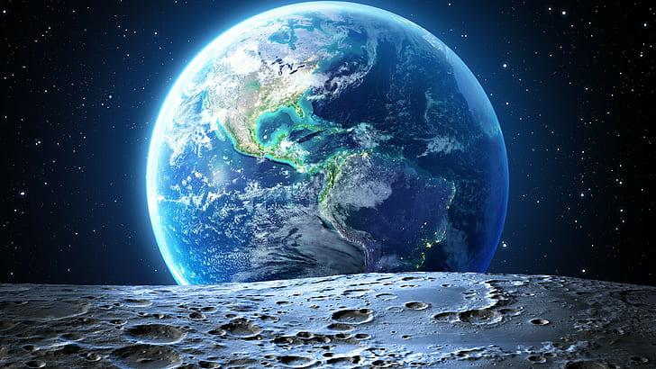
Historical Perspectives and Cultural Significance of Earth’s Mass Measurement
The determination of Earth’s mass represents a convergence of philosophical inquiry, empirical science, and cultural imagination. Early civilizations framed the Earth’s scale within mythological and cosmological narratives, while later scientific revolutions transformed these ideas into measurable quantities. This evolution reflects broader shifts in human understanding—from divine proportions to gravitational constants—and underscores how scientific breakthroughs often emerge from both intellectual curiosity and societal needs. Below, the interplay between ancient cosmologies, foundational experiments, and the cultural reception of these discoveries is examined through historical texts, cross-cultural interpretations, and a chronological milestone analysis.Ancient and Mythological Concepts of Earth’s Scale
Before the advent of quantitative physics, civilizations conceptualized Earth’s "weight" or significance through symbolic and religious frameworks. These perspectives often emphasized harmony, divine balance, or cosmic order rather than mass as a physical property."The Earth is the center of the universe, and all celestial bodies revolve around it in perfect spheres." — Aristotle, On the Heavens (4th century BCE)Aristotle’s geocentric model, rooted in qualitative observations, dominated Western thought for centuries. In contrast, ancient Egyptian and Mesopotamian cosmologies depicted Earth as a stable foundation for the gods, with its "weight" symbolizing permanence. The Enuma Elish (Babylonian creation epic, ~18th century BCE) describes Earth as a "solid disk" supported by primordial waters, reflecting a literal but non-measurable notion of scale.
In Hindu cosmology, the Puranas describe Earth (Prithvi) as one of five elemental bodies (Pancha Mahabhutas), with its mass implicitly tied to the balance of dharma (cosmic order). Chinese I Ching (Book of Changes, ~11th century BCE) associates Earth (Kun) with receptivity and stability, but lacks a numerical framework. These traditions prioritized symbolic weight over empirical measurement, illustrating how pre-scientific cultures framed Earth’s role in universal harmony.
Foundational Texts and Early Scientific Attempts
The transition from qualitative to quantitative Earth-mass estimation began with 17th-century physics, where scholars sought mathematical descriptions of gravitational interactions. Key texts from this era laid the groundwork for later experiments."The force by which the planets are continually drawn off from rectilinear motions and retained in their orbits is that which we endeavor to explain." — Isaac Newton, Philosophiæ Naturalis Principia Mathematica (1687), Book III, Proposition IVNewton’s Principia introduced the inverse-square law of gravitation, enabling theoretical calculations of Earth’s mass if the gravitational constant (G) were known. However, G remained undetermined until the 18th century. Earlier, Johannes Kepler (1619) had described planetary motions without addressing Earth’s mass directly, focusing instead on elliptical orbits.
In 17th-century France, Christiaan Huygens attempted to estimate Earth’s density by comparing the weight of a metal sphere to its volume, but his methods lacked precision. The first empirical approach came from John Michell (1767), who proposed using a torsion balance to measure G, though he died before conducting the experiment. His ideas influenced Henry Cavendish, whose 1798 experiment became pivotal.
Timeline of Key Milestones in Earth’s Mass Measurement
The progression from philosophical speculation to precise measurement spans millennia, marked by technological and theoretical advancements. Below is a chronological overview of critical developments:-
~350 BCE – Aristotle’s Geocentric Model
Aristotle’s qualitative framework dominated Western science, with Earth’s "weight" inferred from its immobility and celestial motions. No numerical mass was proposed. -
1687 – Newton’s Principia and Gravitational Theory
Newton’s laws provided the mathematical tools to calculate Earth’s mass if G were known, but the constant remained elusive. The stage was set for experimental verification. -
1798 – Cavendish Experiment and the Determination of G
Henry Cavendish’s torsion balance experiment measured G with sufficient accuracy to derive Earth’s mass:
Earth’s mass (M) = (gR²)/G, where g = gravitational acceleration at Earth’s surface, R = Earth’s radius, G = gravitational constant.
Cavendish’s result: M ≈ 5.98 × 10²⁴ kg (modern value: 5.972 × 10²⁴ kg). -
1840s – Friedrich Bessel’s Stellar Parallax Refinements
Bessel’s measurements of stellar distances indirectly validated Newtonian gravity, reinforcing Earth’s mass calculations by comparing solar and planetary influences. -
1900s – Einstein’s General Relativity and Post-Newtonian Corrections
Einstein’s theory refined gravitational models, though Earth’s mass remained consistent with Cavendish’s findings. Relativity provided deeper insights into mass-energy equivalence (E=mc²), expanding the context of Earth’s mass. -
1960s–Present – Satellite and Space-Based Measurements
NASA’s GRACE (Gravity Recovery and Climate Experiment, 2002) and GOCE (Gravity Field and Steady-State Ocean Circulation Explorer, 2009) missions achieved sub-centimeter precision in Earth’s gravitational field, updating mass estimates to 5.97219 × 10²⁴ kg (±0.00001%).
The Cavendish Experiment as a Cultural Symbol
Henry Cavendish’s 1798 experiment, though scientifically groundbreaking, also became a cultural touchstone for the public’s perception of scientific inquiry. Conducted in a secluded laboratory at his estate in Clapham, England, the experiment was initially met with skepticism and amusement."The experiment was performed with such nicety that the force could scarcely fail of being perceived." — Henry Cavendish, Philosophical Transactions of the Royal Society (1798)Cavendish’s work was overshadowed by his aristocratic reclusiveness; he was known as the "Human Calculator" for his eccentricity rather than his contributions. The torsion balance’s delicate setup—using a six-foot wire to measure infinitesimal gravitational forces—was described in contemporary journals as "almost magical" in its precision. Public reactions ranged from fascination to ridicule, with satirical cartoons depicting Cavendish as a "mad scientist" tinkering with invisible forces.
The experiment’s cultural legacy lies in its embodiment of the scientific method as a quiet, methodical pursuit—contrasting with the dramatic discoveries of astronomy or chemistry. It also highlighted the collaboration between theory and experiment: Newton’s laws provided the framework, while Cavendish’s ingenuity bridged abstract mathematics with tangible measurement. This duality resonates in modern science communication, where precision experiments like those measuring Earth’s mass are often framed as both intellectually rigorous and culturally transformative.
Advanced Topics: Relativity and Earth’s Mass
General relativity refines classical mass calculations by introducing spacetime curvature, where Earth’s gravitational field is no longer treated as a Newtonian force but as a geometric property of the universe. In high-precision applications—such as satellite navigation systems like GPS—these relativistic corrections are indispensable. The equivalence principle, a cornerstone of Einstein’s theory, posits that gravitational mass (responsible for curvature) and inertial mass (responsible for resistance to acceleration) are identical, a hypothesis Earth’s mass helps empirically validate. Below, the interplay between Earth’s mass, spacetime geometry, and observable phenomena is examined, alongside hypothetical scenarios and mathematical derivations illustrating relativistic effects.Relativistic Adjustments in High-Precision Measurements
Classical mechanics approximates Earth’s mass as a static gravitational source, but general relativity accounts for dynamic spacetime distortions. For instance, GPS satellites orbit at ~20,200 km, where Earth’s gravitational potential (proportional to mass) causes time dilation effects measurable at ~38 microseconds per day. Without relativistic corrections, GPS would accumulate errors of ~10 km daily. The Schwarzschild metric, describing spacetime around a spherically symmetric mass like Earth, adjusts Newtonian gravity by incorporating a term dependent on the mass-energy distribution:Schwarzschild Metric (Simplified):The first term modifies time dilation near Earth’s surface, while the second adjusts radial distances. For a stationary observer at Earth’s surface (\(r = R_E\)), the proper time \(\tau\) differs from coordinate time \(t\) by:
\[
ds^2 = -\left(1 - \frac{2GM}{c^2 r}\right)c^2 dt^2 + \left(1 - \frac{2GM}{c^2 r}\right)^{-1} dr^2 + r^2 d\Omega^2
\]
Where:
\(G\) = gravitational constant, \(M\) = Earth’s mass (~5.97 × 10²⁴ kg), \(c\) = speed of light, \(r\) = radial distance from Earth’s center.
Gravitational Time Dilation:
\[
\frac{d\tau}{dt} = \sqrt{1 - \frac{2GM}{c^2 R_E}} \approx 1 - \frac{GM}{c^2 R_E}
\]
For Earth, this yields a time dilation of ~6.9 × 10⁻¹⁰, or ~0.021 seconds per year at sea level.
Gravitational Mass vs. Inertial Mass and the Equivalence Principle
The equivalence principle asserts that gravitational mass (\(m_g\), determining gravitational force) and inertial mass (\(m_i\), determining resistance to acceleration) are equivalent. Earth’s mass serves as a macroscopic test case: experiments like the Eötvös experiment (1908) and modern torsion balance tests (e.g., MICROSCOPE satellite, 2016) confirm their equivalence to within 1 part in 10¹⁵. This principle underpins general relativity, where mass-energy curvature dictates spacetime geometry.Earth’s role in validating the principle extends to:
Thought Experiment: Hypothetical Alteration of Earth’s Mass
A hypothetical doubling of Earth’s mass (\(M' = 2M\)) would trigger cascading effects across physics, climate, and infrastructure. Below are key consequences derived from relativistic and Newtonian frameworks:-
1. Orbital Mechanics and Tidal Forces
- Moon’s orbit: Period would shrink from ~27.3 days to ~19.3 days, increasing tidal forces by ~41% (proportional to \(M/r^3\)).
- Geostationary satellites: Would require orbits at ~28,500 km (vs. current 42,164 km) to maintain synchronization.
- Increase atmospheric scale height (\(H = kT/mg\)) by a factor of 2, thickening the atmosphere and raising surface pressure to ~2 atm.
- Accelerate weather systems (wind speeds, ocean currents) by \(\sqrt{2}\) due to stronger Coriolis effects.
- Shift the habitable zone inward, potentially rendering Venus-like conditions at Earth’s current distance from the Sun.
- Buildings and bridges: Structural loads would double, requiring reinforced materials (e.g., carbon nanotubes) to prevent collapse.
- Spaceflight: Launch energy would increase by \(\sqrt{2}\) (escape velocity \(v_e = \sqrt{2GM/r}\) becomes \(v_e' = \sqrt{2}v_e\)), making interplanetary travel prohibitively expensive.
- GPS and relativity: Time dilation at Earth’s surface would double, necessitating recalibration of atomic clocks to account for ~0.042 seconds/year of additional dilation.
- Time dilation: Surface observers would experience ~13.8 × 10⁻¹⁰ time dilation (vs. current 6.9 × 10⁻¹⁰), or ~0.042 seconds/year.
- Frame-dragging: Earth’s rotation-induced frame-dragging (Lense-Thirring effect) would strengthen proportionally to mass, altering gyroscope precession rates in satellites.
Earth’s gravitational parameter (\(\mu = GM\)) would double, altering orbital periods via Kepler’s third law:
\[
T^2 \propto \frac{r^3}{\mu} \implies T' = \frac{T}{\sqrt{2}}
\]
2. Climate and Atmospheric Retention
Doubled gravity would:
3. Human Infrastructure and Technology
4. Relativistic Effects
Mathematical Derivation: Earth’s Mass and Gravitational Time Dilation
Gravitational time dilation near Earth’s surface arises from the metric’s time component. For a static observer at radius \(r = R_E\), the proper time \(\tau\) and coordinate time \(t\) relate via:Proper Time in Schwarzschild Geometry:For a satellite at altitude \(h\), the dilation effect weakens:
\[
d\tau = dt \sqrt{1 - \frac{2GM}{c^2 R_E}}
\]
Expanding for small \(GM/(c^2 R_E)\) (valid since \(2GM/(c^2 R_E) \approx 1.4 \times 10^{-9}\)):
\[
d\tau \approx dt \left(1 - \frac{GM}{c^2 R_E}\right)
\]
Integrating over a year (\(t = 1 \text{ year} = 3.15 \times 10^7 \text{ s}\)):
\[
\Delta \tau \approx \Delta t \left(1 - \frac{GM}{c^2 R_E}\right) = \Delta t - \frac{GM \Delta t}{c^2 R_E}
\]
Substituting Earth’s parameters:
\[
\Delta \tau \approx 3.15 \times 10^7 \text{ s} - \frac{(6.674 \times 10^{-11})(5.97 \times 10^{24})(3.15 \times 10^7)}{(3 \times 10^8)^2 (6.371 \times 10^6)} \approx 3.15 \times 10^7 - 0.021 \text{ s}
\]
Thus, a clock at Earth’s surface loses ~0.021 seconds per year relative to a distant observer.
\[
\Delta \tau_h \approx \Delta t \left(1 - \frac{GM}{c^2 (R_E + h)}\right)
\]
GPS satellites (h ≈ 20,200 km) experience opposite dilation (~45 microseconds/day) due to weaker gravity and higher velocity, requiring combined relativistic corrections.
Earth’s mass is more than a static figure; it is a dynamic force that defines the planet’s gravitational pull, magnetic field generation, and even the rhythms of tidal interactions with the Moon. By examining its measurement through historical experiments, modern geophysical models, and relativistic adjustments, we reveal a narrative of scientific progress—one where precision meets innovation. Whether applied to spacecraft navigation, climate modeling, or the redefinition of fundamental units, Earth’s mass remains a testament to humanity’s quest to quantify the unseen forces shaping our world. Understanding this value is not just an exercise in astronomy but a gateway to grasping the intricate balance of planetary systems and the principles governing existence itself.
FAQ
What is the exact mass of Earth in scientific notation?
The mass of Earth is approximately 5.97219 × 10²⁴ kilograms (5.97219e24 kg), as measured by NASA and other space agencies. This value accounts for the planet’s crust, mantle, core, and atmosphere.
How much does Earth weigh in kilograms?
Earth’s mass is 5.97 × 10²⁴ kilograms (5,970,000,000,000,000,000,000,000 kg). This is a standard value derived from gravitational measurements and satellite data.
What are the masses of Earth and the Moon combined?
Earth’s mass is 5.97 × 10²⁴ kg, while the Moon’s mass is 7.34 × 10²² kg. Combined, they total 6.04 × 10²⁴ kg, though the Moon’s mass is only about 1.2% of Earth’s.
What is Earth’s mass and its average radius?
Earth’s mass is 5.97 × 10²⁴ kg, and its average radius is 6,371 kilometers (3,959 miles). The radius varies slightly due to the planet’s oblate shape.
How much does Earth’s atmosphere weigh?
Earth’s atmosphere has a total mass of about 5.15 × 10¹⁸ kg (5.15 quintillion metric tons). This includes all gases, water vapor, and aerosols extending up to the exosphere.
What is Earth’s mass in tons (metric)?
Earth’s mass is 5.97 × 10²¹ metric tons (5,970,000,000,000,000,000 tons). This converts directly from kilograms, as 1 metric ton = 1,000 kg.
Leave a Comment
Comments are moderated before appearing. The data you submit is processed according to the Privacy Policy of Voltefac.