Product in math symbol tracing evolution to modern applications
Table of Contents
- Historical Evolution and Cultural Foundations of Product Symbols in Mathematics
- Ancient and Medieval Notations for Multiplication: A Comparative Timeline
- Symbolic Transition: From Verbal Descriptions to Algebraic Efficiency
- Core Product Symbols in Modern Mathematics
- Multiplication Symbol × (U+00D7)
- Interpunct Symbol · (U+2022 or U+00B7)
- Asterisk Symbol * (U+002A)
- Dot Operator ∙ (U+22C5)
- Juxtaposition (Implicit Multiplication)
- Typographical and Functional Differences Across Disciplines
- Advanced Applications of Product Symbols in Mathematical Systems
- Binary Operations in Group Theory and Abstract Algebra
- Tensor Products in Physics: Quantum Mechanics and General Relativity
- Hadamard Product in Matrix Theory and Machine Learning
- Kronecker Product: Visualization and Computation in Linear Algebra
- Cross Product in 3D Space: Geometric and Algebraic Derivation
- Product Symbols in Programming and Computational Mathematics
- Implicit vs. Explicit Product Symbols and Code Readability
- Comparison of Product Symbols Across Programming Languages
- Rendering Product Symbols in LaTeX and MathJax
Mathematics has long relied on symbols to distill complex ideas into concise expressions, and few operations carry as much weight as the product. From ancient clay tablets to quantum physics equations, the evolution of product symbols reflects humanity’s quest for precision and efficiency in computation. The shift from cumbersome verbal descriptions to streamlined notations like the multiplication dot or the cross mark revolutionized how mathematicians, engineers, and scientists communicate—reducing ambiguity and accelerating discovery across disciplines.
The story of product symbols is one of cultural exchange and innovation, spanning civilizations that shaped modern mathematics. The Egyptians used hieroglyphic-like notations, while Indian scholars introduced the dot as a placeholder for multiplication, later adopted by European mathematicians. Meanwhile, Arabic numerals and Greek geometry laid the groundwork for symbols that now underpin everything from calculus to machine learning algorithms. Understanding this history not only illuminates the roots of mathematical thought but also reveals how symbolic conventions continue to evolve in response to technological and theoretical advances.

Historical Evolution and Cultural Foundations of Product Symbols in Mathematics
The representation of mathematical products has undergone a profound transformation from abstract verbal descriptions to concise symbolic notations, reflecting broader shifts in human cognition, trade, and scientific inquiry. Early civilizations relied on physical objects, tally marks, or cumbersome verbal instructions to convey multiplication concepts, while modern mathematics employs standardized symbols like the multiplication dot (·) or cross (×) to denote operations with unparalleled efficiency. This evolution mirrors the global exchange of mathematical ideas, where cultures like the Egyptians, Greeks, Indians, and Arabs contributed unique notations that laid the groundwork for contemporary algebraic conventions. The transition from repeated addition to symbolic multiplication was not merely a technical advancement but a cultural and linguistic revolution, enabling complex problem-solving in astronomy, commerce, and architecture. Ancient manuscripts, such as the Rhind Mathematical Papyrus (c. 1550 BCE) and the Bakhshali Manuscript (3rd–4th century CE), offer tangible evidence of how early mathematicians encoded multiplication through geometric interpretations and iterative processes. These texts reveal a gradual abstraction of arithmetic operations, where practical needs—such as calculating grain distribution or constructing pyramids—driven the development of symbolic shorthand.
Ancient and Medieval Notations for Multiplication: A Comparative Timeline
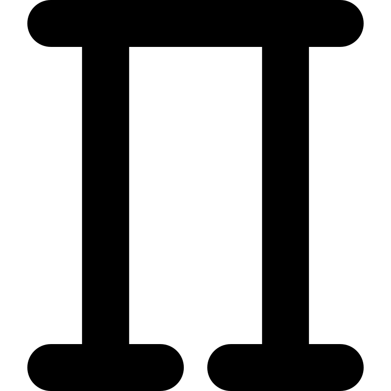 The representation of multiplication varied widely across cultures, often tied to their numeral systems and philosophical approaches to mathematics. While some societies used positional notation (e.g., the Indians with their decimal system), others depended on additive or multiplicative symbols embedded in geometric diagrams. Below is a chronological overview of five pivotal product notations, illustrating their origins, cultural contexts, and eventual obsolescence or adaptation into modern forms.
- Egyptian Multiplication Tables (c. 2000–1000 BCE) The Egyptians employed a method of repeated doubling to simplify multiplication, documented in the Rhind Papyrus. Instead of a dedicated symbol, they used hieroglyphic numerals combined with additive processes. For example, to multiply 13 by 12, they would break it into (8 + 4 + 1) × 12, summing the partial products. This approach reflected their reliance on unit fractions and geometric interpretations of area, where multiplication was visualized as extending lengths or widths.
- Greek Geometric Symbolism (c. 300 BCE–500 CE) Greek mathematicians, including Euclid and Archimedes, represented multiplication implicitly through geometric constructions. In The Elements, Euclid described multiplication as the area of a rectangle with sides a and b, avoiding symbolic notation entirely. The Greeks used diagrams with labeled sides to denote products, a practice that persisted until the late medieval period. For instance, a rectangle with sides marked AB and BC implicitly represented AB × BC.
- Indian Dot Notation (Bakhshali Manuscript, c. 3rd–4th century CE) The Bakhshali Manuscript, discovered in 1881, contains one of the earliest known uses of a dot (·) to denote multiplication, predating European adoption by over a thousand years. Indian mathematicians, such as Brahmagupta (598–668 CE), formalized this notation in their treatises, using it alongside Sanskrit numerals (e.g., a·b for a × b). This innovation stemmed from their advanced decimal system and algebraic traditions, which emphasized symbolic efficiency.
- Arabic Fractional Multiplication (9th–14th century CE) Islamic scholars, particularly in the House of Wisdom (Bayt al-Hikma) in Baghdad, developed notations to handle algebraic equations and fractional multiplication. They used parentheses and word descriptors, such as "multiplied by" (ضرب ḍarab), but avoided dedicated symbols. For example, an equation like x × (a/b) might be written as "x multiplied by a over b." Their work, translated into Latin in the 12th century, influenced European mathematicians to seek more compact representations.
- Medieval European Cross Symbol (16th–17th century CE) The cross (×) as a multiplication symbol emerged in European mathematics during the Renaissance, popularized by Johannes Widmann (1489) in his arithmetic texts. This notation was influenced by commercial accounting practices, where merchants used crosses to denote multiplication in ledgers. However, the cross was initially ambiguous—sometimes confused with the variable x—leading to later alternatives like the dot (·) and implicit juxtaposition (e.g., ab for a × b).
Symbolic Transition: From Verbal Descriptions to Algebraic Efficiency
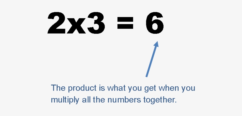 The shift from verbal to symbolic multiplication was catalyzed by the need for clarity, brevity, and scalability in mathematical discourse. Prior to symbolic notation, mathematicians relied on cumbersome phrases like "the product of a and b" or "a multiplied by b", which hindered complex calculations. The adoption of symbols such as the dot (·) or cross (×) allowed for:
- Reduced Ambiguity: Symbols eliminated linguistic variations across languages, ensuring universal comprehension. For example, a·b is instantly recognizable as a product, whereas "a multiplied by b" could be misinterpreted in translations.
- Algebraic Abstraction: Symbols like xy (juxtaposition) or a × b enabled the formulation of generalized equations, a cornerstone of modern algebra. This was critical for advancements in calculus, where Leibniz and Newton used symbolic multiplication to define derivatives and integrals.
- Mechanical Computation: The dot notation (·) became standard in programming and engineering due to its clarity in typed equations, while the cross (×) persisted in educational contexts. The juxtaposition (ab) remains common in variable-based algebra, reflecting its efficiency in polynomial expressions.
- Cross-Cultural Standardization: The International System of Units (SI) and modern scientific publishing adopted the dot (·) to avoid confusion with the variable x, demonstrating how symbolic conventions evolve to meet global needs.
The table below synthesizes these historical notations, highlighting their cultural origins and modern equivalents:
| Symbol | Origin/Culture | Time Period | Modern Equivalent | Example Usage | ||||||||||||||||||||||||||||||||||||||||||||||||||||||
|---|---|---|---|---|---|---|---|---|---|---|---|---|---|---|---|---|---|---|---|---|---|---|---|---|---|---|---|---|---|---|---|---|---|---|---|---|---|---|---|---|---|---|---|---|---|---|---|---|---|---|---|---|---|---|---|---|---|---|
| Hieroglyphic Addition(No dedicated symbol; additive process) | Ancient Egypt | c. 2000–1000 BCE | Repeated addition (e.g., 3 × 4 = 4 + 4 + 4) | Rhind Papyrus: Calculating grain rations via iterative sums. | ||||||||||||||||||||||||||||||||||||||||||||||||||||||
| Geometric Diagrams(Rectangles with labeled sides) | Ancient Greece | c. 300 BCE–500 CE | Area interpretation (e.g., length × width) | Euclid’s Elements: Proving theorems via rectangular areas. | ||||||||||||||||||||||||||||||||||||||||||||||||||||||
| Dot (·)(Brahmi numerals influence) | India (Bakhshali Manuscript) | 3rd–4th century CE | Standard multiplication dot (·) | a·b for a × b in algebraic equations. | ||||||||||||||||||||||||||||||||||||||||||||||||||||||
| Parentheses with Words(e.g., "ضرب" for multiply) | Islamic Golden Age | 9th–14th century CE | Symbolic juxtaposition (ab) | x ضرب (a/b) → Later simplified to x(a/b). | ||||||||||||||||||||||||||||||||||||||||||||||||||||||
| Cross (×)(Commercial ledger influence) | Renaissance Europe | 16th–17th century CE | Dot (·) or juxtaposition (ab)Core Product Symbols in Modern Mathematics
The multiplication operation, fundamental to mathematical and scientific disciplines, relies on a diverse set of product symbols to convey precision, context, and clarity. In contemporary mathematics, these symbols extend beyond the familiar "×" to include implicit notations like juxtaposition, as well as specialized variants tailored for specific fields. Each symbol carries distinct typographical and functional nuances, influencing how equations are interpreted in algebra, calculus, physics, and computer science. This section examines the five most ubiquitous product symbols—×, ·, *, ∙, and juxtaposition—analyzing their usage, formal definitions, and technical distinctions across disciplines. Additionally, it explores the role of Unicode and LaTeX in standardizing these symbols, while addressing common misconceptions that persist in both academic and computational contexts.
Multiplication Symbol × (U+00D7)The symbol × (Unicode U+00D7) is the most visually intuitive representation of multiplication, widely recognized in elementary mathematics and general-purpose contexts. Its origins trace back to the 17th century, introduced by William Oughtred, and it remains the default choice in educational materials and basic arithmetic. In algebra, × is frequently used to denote scalar multiplication, such as in the equation 3 × x = 9, where it explicitly signals the operation between a coefficient and a variable. However, its use diminishes in advanced mathematics due to ambiguity risks—particularly in handwritten or poorly formatted text—where × can resemble the variable x or the letter k. In calculus, × appears in product rule formulations, such as the derivative of f(x) × g(x), though it is often replaced by juxtaposition (e.g., f(x)g(x)) for brevity. In physics, it serves as a clear delimiter in equations involving forces or energy, such as F = m × a, where the distinction between multiplication and vector cross products (denoted by × in a different context) can lead to confusion without proper notation. Computer science largely avoids × in favor of implicit multiplication (e.g., ab in C or ab in MATLAB), as it conflicts with variable naming conventions and lacks support in some programming fonts. Typographical Note: The × symbol is encoded in Unicode as U+00D7 and is rendered in LaTeX via `\times`. Its primary limitation lies in its visual resemblance to other symbols, necessitating contextual clarity in formal writing.Interpunct Symbol · (U+2022 or U+00B7)The · symbol, known as the interpunct or middle dot, serves as a versatile product indicator in mathematics, particularly in linear algebra and physics. Unlike ×, it avoids ambiguity with variables and is favored in contexts where precision is critical. In linear algebra, · is the standard notation for the dot product of two vectors, as seen in a · b = |a||b|cosθ, where it distinguishes the scalar product from the cross product (×). This distinction is vital in signal processing, where the dot product appears in correlation functions and convolution operations, such as in the discrete-time convolution formula:Here, · explicitly marks multiplication within the summation, ensuring clarity in computational implementations. In calculus, · is used in tensor products and functional compositions, such as f · g(x) = f(g(x)), though juxtaposition often suffices. Physics employs · in quantum mechanics to denote inner products of state vectors, e.g., ⟨ψ|φ⟩, where the dot product’s role is implicit but critical. Computer science adopts · in libraries like NumPy (Python) for element-wise multiplication, written as np.dot(a, b), while LaTeX renders it via `\cdot`. Unicode Variants: The interpunct has multiple encodings, including U+2022 (bullet) and U+00B7 (middle dot), with U+22C5 (⋅, dot operator) preferred in mathematical typesetting for consistency. Asterisk Symbol * (U+002A)The asterisk () is ubiquitous in computer science and engineering due to its simplicity and keyboard accessibility. It dominates in programming languages like Python (ab), MATLAB (ab), and SQL (SELECT FROM table), where it explicitly denotes multiplication or concatenation (in strings). In algebra, is less common but appears in formal systems like λ-calculus, where it represents function application (e.g., (λx.x) y). Its ambiguity—serving as both a product symbol and a wildcard in regular expressions—demands contextual interpretation. In calculus, is rarely used, except in convolution integrals (e.g., f g), where it distinguishes the operation from standard multiplication. Physics employs in operator algebra, such as AB for non-commutative products, but this is field-specific. LaTeX renders * via `\ast`, while Unicode provides U+002A (basic asterisk) and U+2217 (∗, asterisk operator) for mathematical contexts. Functional Limitation: The asterisk’s dual role in programming (e.g., ab vs. ab in string repetition) necessitates language-specific conventions, often resolved via syntax rules rather than notation.Dot Operator ∙ (U+22C5)The dot operator (∙) is a refined variant of the interpunct, primarily used in advanced mathematics and engineering to denote scalar multiplication or element-wise operations. In linear algebra, it appears in matrix multiplication definitions, such as:Here, ∙ emphasizes the summation’s multiplicative step, distinguishing it from other operations. Signal processing uses ∙ in discrete convolution, where it clarifies the per-sample multiplication in: In calculus, ∙ is rare but may appear in tensor contractions, while physics reserves it for Hadamard products (element-wise matrix multiplication). LaTeX supports it via `\cdot` or `\middlecdot`, and Unicode encodes it as U+22C5. Typographical Advantage: The ∙ symbol’s centered alignment reduces ambiguity in handwritten or low-resolution text, making it ideal for formal proofs. Juxtaposition (Implicit Multiplication)Juxtaposition—the omission of any product symbol—is the most concise and widely used notation in modern mathematics, particularly in algebra, calculus, and abstract algebra. It arises from the associative property of multiplication, where ab implicitly means a × b. In algebra, this is standard for polynomials (e.g., 3x²y = 3 × x × x × y) and function composition (e.g., f(g(x)) = f ∘ g(x)). Calculus relies heavily on juxtaposition for derivatives (e.g., d/dx (x²) = 2x) and integrals (e.g., ∫x² dx), where symbols like × would clutter notation. In physics, juxtaposition dominates in Newton’s laws (e.g., F = ma) and electromagnetism (e.g., E = kq/r²). Computer science adopts it in mathematical libraries (e.g., NumPy’s ab vs. ab for element-wise operations), though programming languages often require explicit symbols to avoid ambiguity. LaTeX omits any product symbol by default, while Unicode does not encode juxtaposition as a distinct symbol—its meaning is context-dependent. Functional Efficiency: Juxtaposition reduces cognitive load in complex expressions, but its ambiguity in programming (e.g., ab could mean a variable ab or a × b) necessitates language-specific disambiguation rules.Typographical and Functional Differences Across DisciplinesThe choice of product symbol varies significantly across fields due to readability, tradition, and tooling constraints. Below is a comparative analysis of implicit (juxtaposition) and explicit symbols in programming languages and mathematicalAdvanced Applications of Product Symbols in Mathematical SystemsProduct symbols transcend basic arithmetic, serving as foundational tools in abstract structures where operations defy conventional multiplication. In advanced mathematics, these symbols formalize complex interactions—whether in algebraic frameworks, physical theories, or computational models. Their precision enables mathematicians and scientists to model phenomena from quantum entanglement to neural network dynamics, demonstrating how symbolic notation bridges abstract theory and real-world applications. The versatility of product symbols lies in their ability to encode operations that are non-commutative, multi-dimensional, or context-dependent. Below, their roles in abstract algebra, physics, machine learning, and category theory are explored through structured examples and procedural guides.Binary Operations in Group Theory and Abstract AlgebraIn group theory, product symbols like ∘ (composition) define binary operations that satisfy closure, associativity, identity, and invertibility. Unlike arithmetic multiplication, these operations often lack commutativity, requiring explicit notation to distinguish order. For instance, in the symmetric group Sn, the composition ∘ of permutations σ and τ means applying τ first, then σ, written as σ ∘ τ. This notation extends to semigroups and monoids, where associativity (a ∘ (b ∘ c) = (a ∘ b) ∘ c) is preserved but inverses or identities may not exist. Example: The dihedral group Dn (symmetries of a regular n-gon) uses ∘ to combine reflections (ri) and rotations (s), where ri ∘ s yields a distinct symmetry. The non-commutative nature (ri ∘ s ≠ s ∘ rj) underscores the necessity of symbolic clarity. Abstract algebra leverages such symbols to classify structures, solve equations in rings, and analyze automorphisms in field extensions.Tensor Products in Physics: Quantum Mechanics and General RelativityThe tensor product (⊗) is a cornerstone of linear algebra and quantum theory, enabling the combination of vector spaces into higher-dimensional systems. In quantum mechanics, a composite system of particles A and B is represented by the tensor product HA ⊗ HB, where HA and HB are their respective Hilbert spaces. The product state |ψA⟩ ⊗ |ψB⟩ describes correlated quantum states, while entangled states (e.g., Bell states) cannot be factored as simple tensor products. Symbolic Representation in Equations: In Dirac notation, the inner product of two tensor states is written as:⟨φ1⊗φ2 | ψ1⊗ψ2⟩ = ⟨φ1|ψ1⟩ ⟨φ2|ψ2⟩This property extends to quantum gates in circuit models, where a gate UA ⊗ UB acts independently on subsystems. In general relativity, tensor products underpin the spin connection and curvature tensors, where the metric gμν and Christoffel symbols Γλμν are combined via tensor operations to describe spacetime geometry. Hadamard Product in Matrix Theory and Machine LearningThe Hadamard product (∘), or element-wise multiplication of matrices, differs from standard matrix multiplication by avoiding dot products. For matrices A and B of identical dimensions, the Hadamard product is defined as:(A ∘ B)ij = Aij × BijThis operation is pivotal in machine learning, particularly in attention mechanisms of transformer models. In the scaled dot-product attention layer, the attention scores eij are computed as: eij = (Qi KjT) / √dk ∘ maskwhere the Hadamard product with a mask matrix (containing zeros for invalid positions) ensures only valid attention weights contribute to the output. Additionally, Hadamard products appear in recommender systems for element-wise feature scaling and in computer vision for channel-wise multiplications in residual networks. Kronecker Product: Visualization and Computation in Linear AlgebraThe Kronecker product (⊗) constructs a block matrix from two matrices A (size m×n) and B (size p×q), resulting in a mp×nq matrix. Each element aij of A is multiplied by the entire matrix B, arranged in a block structure:A ⊗ B = | a11B a12B ... a1nB | | a21B a22B ... a2nB | | ... ... ... ... | | am1B am2B ... amnB |Step-by-Step Computation: 1. Define Matrices: Let A = [[1, 2], [3, 4]] and B = [[0, 5], [6, 7]]. 2. Block Construction: Multiply each element of A by B: Cross Product in 3D Space: Geometric and Algebraic DerivationThe cross product (×) of two vectors in ℝ³ yields a vector perpendicular to both, with magnitude equal to the area of the parallelogram they span. For vectors a = (a1, a2, a3) and b = (b1, b2, b3), the cross product is computed via the determinant of a symbolic matrix:
Comparison of Product Symbols Across Programming LanguagesThe syntax and precedence of product operations vary significantly across languages, influenced by historical conventions and design goals. Below is a comparison of 10 languages, including syntax, precedence rules, and edge cases:
Edge Cases to Note: Rendering Product Symbols in LaTeX and MathJaxLaTeX and MathJax provide robust tools for rendering product symbols, but misconfigurations can lead to rendering errors. LaTeX uses the `\prod` command for products, while MathJax supports both `\prod` and HTML/CSS-based rendering. Common issues include:Rendered as: \(\prod_{k=1}^n x_k\) Troubleshooting:Symbolic Computation Libraries andThe journey of product symbols in mathematics is more than a chronological account—it is a testament to the power of abstraction in solving real-world problems. Whether in the silent precision of a LaTeX document, the dynamic computations of a Python script, or the theoretical frameworks of abstract algebra, these symbols bridge the gap between abstract concepts and practical applications. As mathematics continues to intersect with fields like artificial intelligence and quantum mechanics, the role of product symbols remains pivotal, proving that even the simplest notations can unlock profound insights and transformative innovations. |
Leave a Comment
Comments are moderated before appearing. The data you submit is processed according to the Privacy Policy of Voltefac.