What Is An Electron Fundamentals Properties And Applications
Table of Contents
- Fundamental Definition and Properties of an Electron
- Electron Properties Compared to Fundamental Particles
- Electrostatic Stabilization in Atomic Systems
- Historical Discovery and Experimental Validation
- Electron Behavior in Atomic and Molecular Systems
- Electron Configurations in Multi-Electron Atoms
- Comparison of Electron Orbital Shapes and Properties
- Electron Sharing and Transfer in Chemical Bonding
- Electron Excitation and Emission in Spectral Lines
- Electrons in Electricity and Conductivity
- Free Electrons and Metallic Conductivity
- Semiconductor Doping and Conductivity Modulation
- Photoelectric Effect and Electron Emission
- Band Theory and Electron Flow in Conductors vs. Insulators
- Electron Applications in Technology
- Electron Beams in Cathode-Ray Tubes and Scanning Electron Microscopes
- Electron-Based Technologies: Role, Principles, and Examples
- Electron Tunneling in Quantum Devices
- Electrons in Lithium-Ion Batteries: Energy Storage Mechanisms
- FAQ
- What is an electronic check?
- What is an electronic signature?
- What is an electron microscope?
- What is an electronic travel authorization?
- What is an electron configuration?
- What is an electron cloud?
Electrons, as fundamental constituents of matter, underpin the behavior of atoms, the flow of electricity, and the operation of modern technologies. Their negative charge and quantum properties govern chemical bonding, electronic conductivity, and even the emission of light in spectral lines. From J.J. Thomson’s groundbreaking experiments to their pivotal role in semiconductors and quantum devices, electrons exemplify the intersection of physics and innovation. This exploration examines their defining characteristics, atomic interactions, and transformative applications across science and engineering.
At the heart of atomic structure, electrons balance protons’ positive charge through electrostatic forces, stabilizing matter while enabling diverse physical phenomena. Their wave-particle duality challenges classical intuition, yet it unlocks technologies from cathode-ray tubes to MRI machines. By dissecting their properties—charge, mass, spin—and their behavior in bonds, conductivity, and quantum tunneling, we reveal how these subatomic particles shape both natural systems and human innovation. The journey from theoretical discovery to practical applications underscores their indispensable role in modern science.
Fundamental Definition and Properties of an Electron
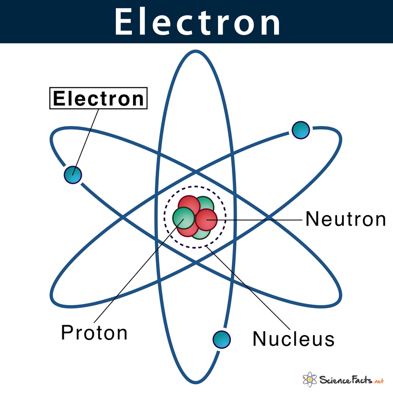
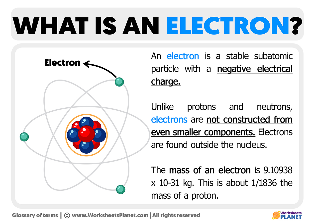
Electrons are fundamental subatomic particles characterized by a negative electric charge, negligible rest mass relative to protons and neutrons, and a quantum property known as spin. As the lightest stable charged particles, they occupy discrete energy levels within atoms, defining chemical behavior, bonding, and electromagnetic interactions. Their role extends beyond atomic structure to electronics, magnetism, and quantum mechanics, where their wave-particle duality underpins modern technologies.
Electrons are essential constituents of matter, governing atomic stability through electrostatic attraction to positively charged protons in the nucleus. Their properties distinguish them from other fundamental particles, including quarks (constituents of protons/neutrons) and positrons (antiparticles of electrons). Below, a comparative analysis highlights key differences, while Coulomb’s law illustrates their stabilizing influence in atomic systems.
Electron Properties Compared to Fundamental Particles
The following table summarizes the fundamental properties of electrons, protons, and quarks, emphasizing their charge, mass, and spin. Values are derived from the CODATA 2018 recommendations, ensuring precision in subatomic physics.| Particle | Charge (Coulombs) | Mass (kg) | Spin (ħ units) |
|---|---|---|---|
| Electron (e⁻) | -1.602176634 × 10⁻¹⁹ C | 9.1093837015 × 10⁻³¹ kg | ½ |
| Proton (p⁺) | +1.602176634 × 10⁻¹⁹ C | 1.67262192369 × 10⁻²⁷ kg | ½ |
| Up Quark (u) | +⅔ × 1.602176634 × 10⁻¹⁹ C | 2.2 × 10⁻³⁰ kg (approximate) | ½ |
| Down Quark (d) | -⅓ × 1.602176634 × 10⁻¹⁹ C | 4.7 × 10⁻³⁰ kg (approximate) | ½ |
Electrons exhibit a 1836-fold lower mass than protons, enabling their mobility within atomic orbitals. Their spin-½ classification as fermions adheres to the Pauli exclusion principle, restricting multiple electrons to identical quantum states. In contrast, quarks—bound by the strong nuclear force—possess fractional charges and masses influenced by quantum chromodynamics (QCD).
Electrostatic Stabilization in Atomic Systems
The stability of atoms arises from the balance between the electrostatic attraction between electrons and protons and the centrifugal force due to electron motion. In the hydrogen atom (the simplest system), this equilibrium is governed by Coulomb’s law, which quantifies the electrostatic force between two point charges:Coulomb’s Law:Step-by-Step Application in Hydrogen:
\( F = k_e \frac{|q_1 q_2|}{r^2} \)
where:
\( F \) = electrostatic force (N), \( k_e \) = Coulomb’s constant (8.9875 × 10⁹ N·m²/C²), \( q_1, q_2 \) = charges of electron and proton, \( r \) = distance between charges.
1. Charge Interaction: The electron’s negative charge (\(-e\)) and the proton’s positive charge (\(+e\)) create an attractive force proportional to \( \frac{e^2}{r^2} \).
2. Quantization of Orbits: Electrons occupy discrete energy levels (n = 1, 2, 3...) due to Bohr’s model, where the centripetal force balances Coulombic attraction:
\( \frac{m_e v^2}{r} = \frac{e^2}{4 \pi \epsilon_0 r^2} \)
(Simplified for hydrogen, ignoring relativistic effects.)
3. Ground State Stability: At \( n = 1 \), the electron’s average distance (\( r \approx 5.29 \times 10^{-11} \) m, the Bohr radius) minimizes energy while preventing collapse via the Heisenberg uncertainty principle.
4. Multi-Electron Atoms: In systems with \( Z > 1 \), electron-electron repulsion (shielding) modifies effective nuclear charge, explained by Slater’s rules or density functional theory (DFT).
Real-World Implications:
The electrostatic binding energy of electrons determines atomic spectra (e.g., hydrogen’s Lyman series) and chemical reactivity. Disruptions in this balance—such as in ionization or excited states—underlie phenomena like fluorescence and semiconductor behavior.
Historical Discovery and Experimental Validation
The electron’s existence was inferred through a series of 19th- and early 20th-century experiments, culminating in its formal identification as a fundamental particle. Below is a chronological timeline of key milestones:Timeline of Electron Discovery:Legacy of Experiments:
1838 – Michael Faraday observes "electrical particles" during electrolysis, hinting at discrete charge carriers.
1874 – George Johnstone Stoney coins the term "electron" to describe the smallest unit of electric charge (\( e \)).
1897 – J.J. Thomson conducts cathode ray experiments, measuring the charge-to-mass ratio (\( e/m \)) of electrons via deflection in electric/magnetic fields. His work confirms electrons as subatomic constituents.
1909 – Robert Millikan performs the oil-drop experiment, determining the electron’s absolute charge (\( e = -1.602 \times 10^{-19} \) C) through precise measurements of falling charged droplets.
1913 – Niels Bohr integrates electrons into atomic theory via his model of quantized orbits, resolving the hydrogen spectrum puzzle.
1924 – Louis de Broglie proposes electron wave-particle duality, later validated by Davisson-Germer’s diffraction experiments (1927).
1932 – Carl Anderson discovers the positron (electron’s antiparticle), confirming Dirac’s relativistic quantum mechanics predictions.
Thomson’s and Millikan’s work provided empirical foundations for quantum mechanics, while later discoveries (e.g., positrons) expanded the Standard Model. The electron’s role in quantum tunneling (e.g., scanning tunneling microscopy) and superconductivity further underscores its centrality to modern physics.
Electron Behavior in Atomic and Molecular Systems
Electrons govern the chemical and physical properties of matter by occupying quantized energy states within atoms and forming bonds between atoms. In multi-electron systems, their arrangement follows strict quantum mechanical rules, determining reactivity, bonding types, and spectral characteristics. This section explores electron configurations in atoms, orbital interactions in molecules, and the dynamic processes of electron excitation and emission, with a focus on empirical models and experimental observations.Electron Configurations in Multi-Electron Atoms
The distribution of electrons across atomic orbitals in multi-electron systems adheres to three foundational principles: the Aufbau principle, Pauli exclusion principle, and Hund’s rule. These govern the stability, energy ordering, and spatial arrangement of electrons, influencing atomic properties such as ionization energy and electron affinity.Aufbau Principle
Electrons fill orbitals in order of increasing energy, following the sequence: 1s < 2s < 2p < 3s < 3p < 4s < 3d < 4p, etc. This principle is derived from experimental observations of atomic spectra and quantum mechanical calculations. For example:
Pauli Exclusion Principle
No two electrons in an atom can occupy the same quantum state (defined by n, l, mₗ, mₛ). This restricts each orbital to a maximum of two electrons with opposite spins (↑↓). Violations of this principle lead to unstable configurations, as seen in helium’s 1s² ground state.
Hund’s Rule
When filling degenerate orbitals (e.g., 2pₓ, 2pᵧ, 2p_z), electrons maximize spin multiplicity by occupying separate orbitals singly before pairing. This minimizes electron-electron repulsion and stabilizes the atom. For instance, nitrogen’s 2p³ configuration features three unpaired electrons, whereas oxygen’s 2p⁴ pairs two electrons in one orbital.
Comparison of Electron Orbital Shapes and Properties
Orbital shapes dictate electron probability distributions and chemical behavior. The following table summarizes key characteristics of s, p, d, and f orbitals, including their spatial geometry, electron capacity, and energy level examples.| Orbital Type | Shape Description | Max Electrons | Energy Level Example |
|---|---|---|---|
| s | Spherically symmetric; highest probability density at the nucleus. | 2 | 1s (Hydrogen ground state), 2s (Lithium valence orbital) |
| p | Dumbbell-shaped; oriented along x, y, or z axes (pₓ, pᵧ, p_z). | 6 | 2p (Carbon’s valence orbitals), 3p (Phosphorus) |
| d | Cloverleaf or double-dumbbell; five distinct orientations (dₓᵧ, dᵧ_z, etc.). | 10 | 3d (Transition metals like Scandium), 4d (Yttrium) |
| f | Complex shapes with multiple lobes; seven possible orientations. | 14 | 4f (Lanthanides like Cerium), 5f (Actinides like Uranium) |
In multi-electron atoms, orbital energies deviate from the hydrogen-like model due to electron-electron repulsion and nuclear shielding. For example:
Electron Sharing and Transfer in Chemical Bonding
Electrons mediate interactions between atoms through covalent bonds (shared electrons) and ionic bonds (transferred electrons). These processes are visualized using Lewis structures and electron density maps, which illustrate spatial distributions and bonding characteristics.Covalent Bonding in Molecules
Electrons are shared between atoms to achieve stable electron configurations. For example:
Ionic Bonding and Electron Transfer
Complete transfer of electrons between atoms with large electronegativity differences (e.g., metals and nonmetals) forms ionic compounds. For instance:
Electron Density Maps and Lewis Structures
Electron Excitation and Emission in Spectral Lines
Electrons transition between discrete energy levels when absorbing or emitting photons, producing atomic spectra characteristic of each element. The hydrogen spectrum serves as a foundational model for understanding these processes, governed by the Rydberg formula:\[Flowchart of Electron Transitions and Photon Emission
\frac{1}{\lambda} = R_H \left( \frac{1}{n_1^2} - \frac{1}{n_2^2} \right)
\]
where:
\(\lambda\) = wavelength of emitted/absorbed light, \(R_H\) = Rydberg constant (1.097 × 10⁷ m⁻¹), \(n_1\), \(n_2\) = principal quantum numbers (\(n_2 > n_1\)).
The following process describes electron excitation and subsequent emission in hydrogen-like systems:
1. Ground State (n=1): Electron occupies the lowest energy level.
2. Absorption: Photon energy (\(E = h\nu\)) excites the electron to a higher level (e.g., n=2 or n=3).
3. Metastable State: Electron resides in an excited state for ~10⁻⁸ seconds before relaxing.
4. Emission: Electron transitions back to a lower level, releasing a photon with energy \(E = h\nu = E_{n_2} - E_{n_1}\).
Real-World Applications
Electrons in Electricity and Conductivity
The efficiency of electron transport depends on the balance between electron mobility and scattering mechanisms, including phonon interactions and impurities. Semiconductors leverage doping techniques to engineer conductivity, enabling applications in electronics and photonics. Meanwhile, the photoelectric effect demonstrates how electron emission from surfaces varies with material properties, illustrating the quantum nature of light-matter interactions.
Free Electrons and Metallic Conductivity
Metallic conductivity arises from the delocalized valence electrons in a metal lattice, which form a Fermi gas obeying quantum statistical mechanics. These free electrons move under an applied electric field, contributing to current flow according to Ohm’s law (V = IR), where resistance (R) is influenced by electron scattering events. Key scattering mechanisms include:The Drude model quantifies resistivity as:
ρ = m / (n e² τ), where:In real metals, deviations from Ohm’s law occur at high fields (non-linear I-V curves) or low temperatures (quantum interference effects).
m = electron effective mass, n = electron density, e = electron charge, τ = mean free time between collisions.
Semiconductor Doping and Conductivity Modulation
Semiconductors exhibit controlled conductivity through doping, where intentional impurities introduce excess electrons (n-type) or holes (p-type). The process alters carrier concentration and Fermi level, enabling tailored electrical properties. Below is a comparative table of intrinsic and extrinsic semiconductors:| Property | Intrinsic | n-type | p-type |
|---|---|---|---|
| Majority carriers | Electrons and holes (equal) | Electrons | Holes |
| Doping atoms | None | Donors (e.g., P, As in Si) | Acceptors (e.g., B, Ga in Si) |
| Fermi level position | Mid-bandgap | Near conduction band | Near valence band |
| Conductivity mechanism | Thermal excitation | Donor ionization | Acceptor ionization |
| Example materials | Pure Si, Ge | Phosphorus-doped Si | Boron-doped Si |
1. Substrate selection: High-purity silicon or germanium (bandgap ~1.1 eV for Si, ~0.7 eV for Ge).
2. Impurity introduction: Thermal diffusion or ion implantation of dopants (e.g., phosphorus for n-type).
3. Activation: Annealing to repair lattice damage and electrically activate dopants.
4. Carrier concentration control: Adjusting dopant concentration alters conductivity (σ = n e μ, where μ = mobility).
Photoelectric Effect and Electron Emission
The photoelectric effect describes electron emission from a material surface when illuminated by light of sufficient energy. Einstein’s equation (E = hν) establishes the threshold condition:hν = Φ + KE_max, where:Key observations:
h = Planck’s constant (6.626 × 10⁻³⁴ J·s), ν = incident light frequency, Φ = work function (material-dependent), KE_max = maximum kinetic energy of emitted electrons.
Graph sketch description:
Band Theory and Electron Flow in Conductors vs. Insulators
Band theory explains electrical conduction by dividing electron energy states into valence bands (filled at T = 0 K) and conduction bands (empty in insulators). The bandgap (E_g) determines material classification:Key differences in electron flow:Band structure implications:
Conductors: High electron mobility (μ ≈ 10⁻³–10⁻² m²/V·s) due to partially filled bands. Insulators: Near-zero mobility (μ ≈ 10⁻¹⁰ m²/V·s) with fully occupied valence bands. Semiconductors: Intermediate mobility (μ ≈ 10⁻³ m²/V·s), tunable via doping or temperature.
Electron Applications in Technology
Electrons serve as the foundational building blocks of modern technology, enabling innovations from display systems to energy storage and quantum computing. Their controlled manipulation—through electric fields, magnetic lenses, or quantum tunneling—drives the functionality of devices ranging from household electronics to medical imaging equipment. Below are key applications where electron behavior is harnessed to achieve precision, efficiency, and novel functionalities at microscopic and macroscopic scales.Electron Beams in Cathode-Ray Tubes and Scanning Electron Microscopes
Electron beams are directed streams of electrons generated under high vacuum, accelerated by electric potentials, and focused using electromagnetic lenses. These beams are critical in imaging and material analysis due to their high resolution and ability to interact with matter at nanometer scales.Cathode-Ray Tubes (CRTs)
In CRTs, electrons emitted from a heated cathode are accelerated toward a phosphor-coated screen by an anode voltage (typically 10–30 kV). Magnetic deflection coils steer the beam horizontally and vertically, creating a raster pattern that illuminates pixels on the screen. The accelerating voltage determines beam energy, influencing penetration depth and brightness, while magnetic lenses (via Helmholtz coils) refine focus to minimize spot size. CRTs were pivotal in early televisions and computer monitors, though modern flat-panel displays have largely replaced them due to superior efficiency and compactness.
Scanning Electron Microscopes (SEMs)
SEMs utilize electron beams to scan surfaces with resolutions down to 1–10 nm. Electrons are emitted from a tungsten or field-emission source, accelerated by voltages of 0.5–30 kV, and focused via electromagnetic lenses into a fine probe. As the beam raster-scans the sample, emitted secondary or backscattered electrons are detected to construct a high-resolution 3D image. Magnetic lenses adjust beam convergence, while stigmators correct astigmatism to ensure sharp imaging. SEMs are indispensable in materials science, failure analysis, and nanotechnology for inspecting surface morphology and composition.
Electron-Based Technologies: Role, Principles, and Examples
Electrons enable diverse technologies by participating in charge transport, photon emission, or quantum phenomena. The following table summarizes key applications, their electron-driven mechanisms, underlying principles, and real-world implementations.| Technology | Electron Role | Key Principle | Real-World Example |
|---|---|---|---|
| Light-Emitting Diodes (LEDs) | Recombination of electrons and holes in semiconductor junctions releases photons. | Electroluminescence: Energy bandgap transition emits light when electrons drop from conduction to valence bands. | Solid-state lighting (e.g., Philips Hue smart bulbs), automotive indicators, and full-color displays. |
| Transistors | Controlled flow of electrons between source and drain via a gate electrode. | Field-effect modulation: Voltage applied to the gate alters the conductive channel’s width, enabling switching or amplification. | Microprocessors (e.g., Intel Core i9 CPUs), memory chips (DRAM), and power management ICs. |
| Magnetic Resonance Imaging (MRI) | Electrons in hydrogen nuclei (protons) precess in a magnetic field, emitting radio-frequency signals. | Nuclear magnetic resonance (NMR): Spin excitation and relaxation of protons generate contrast in soft tissues. | Medical diagnostics (e.g., Siemens MAGNETOM Skyra 3T scanners for brain and cardiac imaging). |
| Photovoltaic Cells | Absorption of photons excites electrons from valence to conduction bands, generating electric current. | Photoelectric effect: Semiconductor materials (e.g., silicon) create electron-hole pairs under illumination. | Solar panels (e.g., SunPower Maxeon series for residential and utility-scale installations). |
| Vacuum Tubes | Thermionic emission of electrons from a heated cathode to an anode, modulated by grids. | Space-charge-limited current: Electron flow is controlled by electrostatic fields in a vacuum. | Amplifiers (e.g., vintage audio equipment like the Fender Twin Reverb guitar amplifier). |
Electron Tunneling in Quantum Devices
Electron tunneling exploits the quantum mechanical probability of particles traversing energy barriers thinner than their de Broglie wavelength, enabling technologies that defy classical physics. This phenomenon is governed by the decay of the wavefunction’s probability amplitude across the barrier, described by:The tunneling probability amplitude for an electron encountering a potential barrier of height \( V_0 \) and width \( d \) is given by:Flash Memory
\[ \psi(x) = \psi_0 e^{-kx} \]
where \( k = \sqrt{\frac{2m(V_0 - E)}{\hbar^2}} \), \( m \) is the electron mass, \( E \) is the electron energy, and \( \hbar \) is the reduced Planck constant. For \( E < V_0 \), electrons have a non-zero probability of appearing on the opposite side of the barrier.
In flash memory, electrons tunnel through a thin oxide layer (typically 10 nm) from a floating gate to a control gate, altering the transistor’s threshold voltage. Applying a high voltage injects electrons into the floating gate, storing data as a binary state (1 or 0). Reading involves sensing the current flow, while erasing requires tunneling electrons back to the substrate. This non-volatile storage is used in USB drives, SSDs, and smartphones (e.g., Samsung EVO Plus SSDs).
Scanning Tunneling Microscopes (STMs)
STMs leverage tunneling currents between a sharp metal tip and a conductive surface to map atomic-scale topography. By maintaining a constant current (via feedback loops adjusting tip height), the instrument traces electron density variations with sub-ångström precision. STMs revolutionized surface science, enabling atomic manipulation (e.g., IBM’s 2012 "STIBM" logo etched with xenon atoms) and material characterization.
Electrons in Lithium-Ion Batteries: Energy Storage Mechanisms
Lithium-ion batteries store energy through reversible intercalation of lithium ions and electron transfer between electrodes, facilitated by an electrolyte. The process involves three core stages: lithium extraction at the anode, ion transport through the electrolyte, and lithium insertion at the cathode.Anode Reaction (Lithium Intercalation)
During discharge, lithium atoms in the graphite anode lose electrons, forming \( \text{Li}^+ \) ions and releasing them into the electrolyte:
\[ \text{Li}_x\text{C}_6 \rightarrow x\text{Li}^+ + x e^- + 6\text{C} \]
The electrons travel through the external circuit to the cathode, while \( \text{Li}^+ \) ions migrate via the electrolyte (e.g., lithium hexafluorophosphate in organic solvents). Common anodes include graphite (theoretical capacity: 372 mAh/g) or silicon composites for higher energy density.
Electrolyte Transport
The electrolyte, a lithium salt dissolved in a non-aqueous solvent (e.g., ethylene carbonate), must dissociate \( \text{Li}^+ \) ions while blocking electron flow to prevent short circuits. Polymer or gel electrolytes are used in solid-state batteries to enhance safety and flexibility. Ion mobility is optimized by maintaining a porous separator between electrodes.
Cathode Reaction (Lithium Insertion)
At the cathode (e.g., lithium cobalt oxide, \( \text{LiCoO}_2 \)), \( \text{Li}^+ \) ions intercalate into the layered structure, paired with electron acceptance:
\[ \text{Li}_{1-x}\text{CoO}_2 + x\text{Li}^+ + x e^- \rightarrow \text{LiCoO}_2 \]
This reaction reverses during charging, extracting lithium ions back to the anode. Cathode materials like lithium iron phosphate (\( \text{LiFePO}_4 \)) offer thermal stability and longer cycle life, while nickel-manganese-cobalt oxides (NMC) balance energy density and power.
Electron Transport Pathway
Electrons flow from the anode to the cathode through the external circuit, driving current to power devices. The battery’s voltage (typically 3.6–4.2 V per cell) is determined by the electrochemical potential difference between the two electrodes. Modern batteries incorporate protective circuits to prevent overcharging or deep discharge, which can degrade materials or cause thermal runaway.
Electrons emerge as the linchpin of atomic stability, electrical conduction, and technological advancement, bridging abstract theory with tangible progress. Their discovery reshaped our understanding of matter, while their manipulation in semiconductors, batteries, and imaging devices continues to drive innovation. From the precision of quantum mechanics to the ubiquity of electronic devices, electrons exemplify how fundamental science translates into transformative applications. As research pushes boundaries—whether in nanoscale electronics or energy storage—their role remains central to unlocking future possibilities, cementing their status as one of nature’s most influential particles.
FAQ
What is an electronic check?
An electronic check (e-check) is a digital version of a traditional paper check, processed electronically between banks. It uses the same routing and account numbers but is transmitted via ACH (Automated Clearing House) networks instead of being physically written or mailed. Businesses and individuals commonly use them for payments, reducing paper handling and processing time.
What is an electronic signature?
An electronic signature is a legally binding digital version of a handwritten signature, created using encryption or authentication methods. It can be a scanned image, a typed name, or a dynamic signature captured via software, and it confirms the signer’s intent to agree to a document. Many countries recognize them under eIDAS or similar laws for contracts and transactions.
What is an electron microscope?
An electron microscope is a high-powered imaging tool that uses a beam of electrons (instead of light) to magnify objects at nanoscale resolutions, often thousands of times smaller than what’s visible with a light microscope. There are two main types: transmission (TEM) and scanning (SEM) electron microscopes, used in materials science, biology, and nanotechnology to study surfaces and internal structures.
What is an electronic travel authorization?
An electronic travel authorization (ETA) is an online permission required by some countries (like Australia or Canada) for visa-exempt travelers before boarding a flight. It’s submitted via a government website, typically costs a small fee, and is linked to the passenger’s passport. Approval is usually granted quickly, allowing entry for tourism or business without a traditional visa.
What is an electron configuration?
Electron configuration describes how electrons are distributed among the atomic orbitals of an atom, following rules like the Aufbau principle, Pauli exclusion, and Hund’s rule. It’s written using notation (e.g., 1s² 2s² 2p⁶) to show which energy levels and subshells are occupied, determining an element’s chemical properties and reactivity. The configuration follows the periodic table’s structure, with electrons filling orbitals in order of increasing energy.
What is an electron cloud?
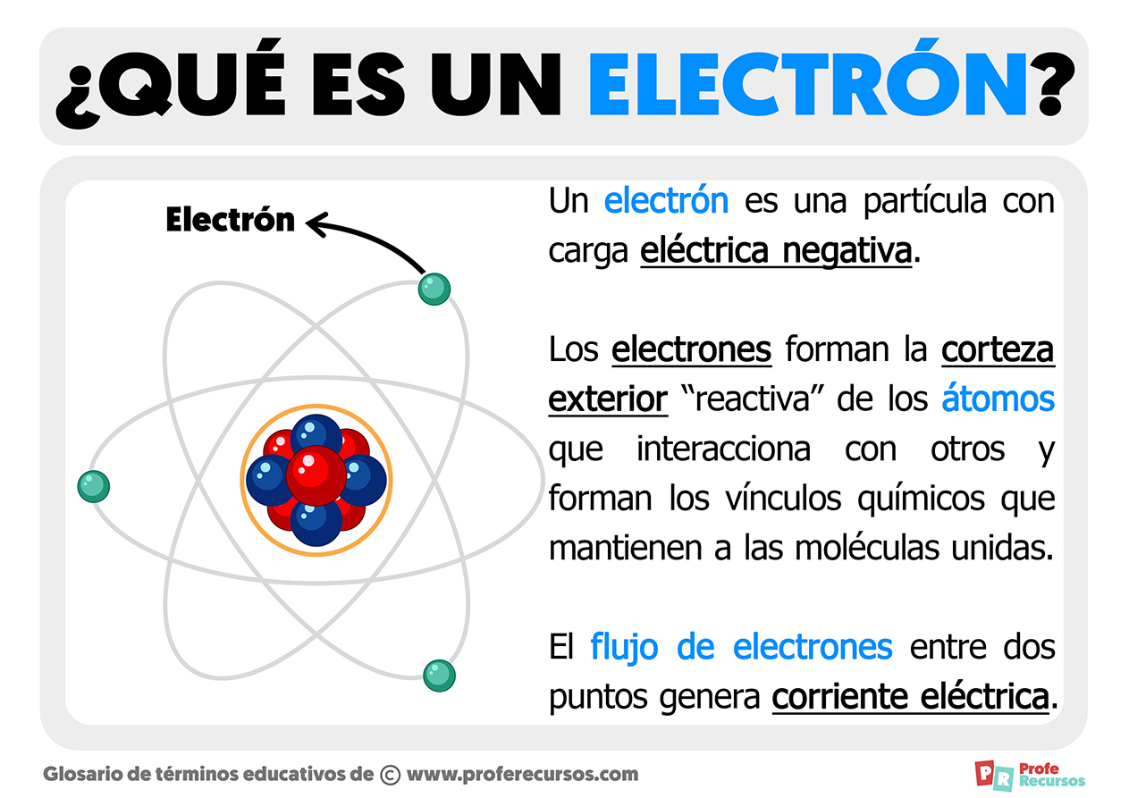
The electron cloud is a visual model representing the probable locations of electrons around an atom’s nucleus, based on quantum mechanics. Unlike fixed orbits, it shows regions (orbitals) where electrons are likely to be found, with varying densities indicating probability. This model explains chemical bonding and atomic behavior, as electrons aren’t confined to precise paths but exist in fuzzy, energy-defined zones.
Leave a Comment
Comments are moderated before appearing. The data you submit is processed according to the Privacy Policy of Voltefac.